Technical data

94
Chapter 5: Fortran Enhancements for Multiprocessors
Example 2: Trade-Offs
Sometimes you must choose between the possible optimizations and their
costs. Look at the following code segment:
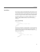
DO J = 1, N
DO I = 1, M
A(I) = A(I) + B(J)*C(I,J)
END DO
END DO
This loop can be parallelized on I but not on J. You could interchange the
loops to put I on the outside, thus getting a bigger work quantum.
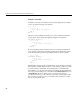
C$DOACROSS LOCAL(I,J)
DO I = 1, M
DO J = 1, N
A(I) = A(I) + B(J)*C(I,J)
END DO
END DO
However, putting J on the inside means that you will step through the C
array in the wrong direction; the leftmost subscript should be the one that
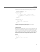
varies the fastest. It is possible to parallelize the I loop where it stands:
DO J = 1, N
C$DOACROSS LOCAL(I)
DO I = 1, M
A(I) = A(I) + B(J)*C(I,J)
END DO
END DO
but M needs to be large for the work quantum to show any improvement. In
this particular example, A(I) is used to do a sum reduction, and it is possible
to use the reduction techniques shown in Example 4 of “Breaking Data
Dependencies” on page 85 to rewrite this in a parallel form. (Recall that there
is no support for an entire array as a member of the REDUCTION clause on
a DOACROSS.) However, that involves converting array A from a
one-dimensional array to a two-dimensional array to hold the partial sums;
this is analogous to the way we converted the scalar summation variable
into an array of partial sums.