Doc-It® Life Science Software Installation and User Instructions Doc-It®LS Image Acquisition Software Doc-It®LS Image Analysis Software UVP, LLC 2066 W 11th Street, Upland, CA 91786 Tel: (800) 452-6788 / (909) 946-3197 Fax: (909) 946-3597 Email: info@uvp.com Ultra-Violet Products Ltd Unit 1, Trinity Hall Farm Estate Nuffield Road, Cambridge CB4 1TG UK Tel: +44(0)1223-420022 / Fax: +44(0)1223-420561 Email: uvp@uvp.co.uk Web site: uvp.
Table of Contents Introduction.................................................................................................................................................... 1 Welcome .................................................................................................................................................... 1 Minimum System Requirements ................................................................................................................
Overview .................................................................................................................................................. 37 Filter Navigation ....................................................................................................................................... 37 Filter Menu ............................................................................................................................................... 37 Filter Plugins ......................
Navigating 1D Analysis ............................................................................................................................ 60 1D Analysis Plugin Module ...................................................................................................................... 60 1D Analysis Context Menu Commands ................................................................................................... 62 Finding Lanes and Bands ....................................................
Printing Image History............................................................................................................................ 101 Print ........................................................................................................................................................ 102 Supporting 21 CFR Part 11 Compliance ................................................................................................... 103 Purpose .................................................
Introduction Introduction Welcome Life Science (LS) software from UVP lets users acquire, enhance, and analyze images in a simple and efficient way. The software is designed to image electrophoresis gels (DNA, RNA, Protein), blots, membranes, plates, plants, and animals. Once the image has been captured with an application-specific camera, it can be saved for record keeping purposes, manipulated for analysis, and annotated to point out key features.
Introduction Minimum System Requirements Windows XP Professional with Service Pack-2 or higher (32 bit only), Vista (32 bit only), or Windows 7 (32 bit only) Internet Explorer 6.0 or higher [To determine the version of Internet Explorer, open Internet Explorer and click on Help > About] Intel Pentium Processor or equivalent, 1.
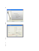
Introduction On the Fly Activation To immediately activate the software through the Internet: Choose On the fly activation. If the computer is not connected to the Internet, follow the instructions for Offline activation or call UVP to register the software. Click Next to continue. Complete all required information on the form. Fill out the Serial Number located on the CD. The number should be four sets of six numbers. Click the Get Activation No.
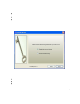
Introduction Offline Activation Select Offline Activation if the computer is not connected to the Internet. This allows the user to obtain the activation code and enter it at another time. Click Next to continue. Click the link provided and complete the form to obtain instructions. Click Finish. Single-User License Single-user license allows the software to be used on a single computer. A Welcome to the Licensing Wizard window will appear. Select the Single client access license option, and select Next.
Introduction This system of usernames and passwords is separate from the one that is used to login to the computer. Setting up user accounts is mandatory if support for CFR 21 Part 11 is required from the software. If individual accounts are not required, create just one account for all users and give full permissions to that account. Enable secure user accounts Request a System Administrator to log into the Windows computer.
Introduction Enter a password. On initial installation, a screen will pop up to request a password and password confirmation. A password is required. Click Login. Adding a New User From the menus, click Tools > User Administration to open the User Administration window. Click the New User button, type in the user name and password. Type in the new user name and password. Each time the new user logs in, use that new user name and password.
Introduction Users Rights Depending on the privileges for the user that has logged onto windows, the following rights are available to that user for the software: Login Privileges Rights Install Un-Install Open and Run User Administration Use the Camera Restricted X* X Standard/Power X* X Admin X X X X X X = Supported rights. Note that even though a user may be able to do things with the software which are outside of this matrix, UVP neither recommends it, nor supports it.
Introduction License Agreement End User License Agreement PLEASE READ THE FOLLOWING AGREEMENT CAREFULLY This Agreement is between UVP, LLC of 2066 West 11th Street, Upland, California 91786 (hereinafter "Licensor") and the end user of UVP software (hereinafter "Licensee").
Introduction Limited Warranty and Disclaimer Licensor warrants the software and related documentation to be free from defects in materials and workmanship, under normal use for a period of ninety (90) days from the date of purchase as evidenced by a copy of the sales receipt or packing slip.
Navigating the Software Navigating the Software Main Window - Shows the full software screen Menus - Discusses the menus available Toolbars - Discusses the tollbars and the ability to rearrange the tool buttons Plug-In Modules - Several plug-in modules are provided as user-friendly interfaces for specific software tasks; this section discusses the various modules and the ability to position the modules Image Windows - Discusses the use of image windows in the workspace Main Window After the LS software is
Navigating the Software NOTE: Although most commands appear on the menus, some features are only available through the Plug-in Modules. If the Plug-in Modules are hidden, they can be shown by selecting the modules from View > Plug-ins whenever needed. Analysis Menu: Contains modules to perform Colony Counting, 1D Analysis and Area Density.
Navigating the Software Cut: Cuts a specific area Undo: Reverses the last command Redo: Repeats the last command Arrow: Selects an annotation to edit Text Tool: Text annotation Line, Rectangle, Ellipse and Highlighter Tools: Annotation tools Define Image Scale: Allows users to set the scale for images Measure Length: Measures the distance between any two points on the image, units depend on spatial calibration Measure Angle: Measures an angle Measure Area: Measures an area on the image New ROI: Removes t
Navigating the Software Rearranging Toolbars The order of the individual toolbar sections can be rearranged by placing the mouse arrow over the dotted line at the edge of each toolbar section and moving the toolbar. The default position of the toolbars is located horizontally below the menus. The toolbars may be moved to the bottom of the screen or vertically on the left or right side. Each section can be deleted or added back by clicking View > Toolbars and select the toolbars to display on the screen.
Navigating the Software Showing the Image in Actual Size To show the image in actual size (no scaling), choose View > Zoom. Set the zoom factor to 100%. Or click the right mouse button on the image and select View Original Size. Images taken at high resolution will look large on the screen. Fitting the Image to the Window To show the entire image in the window (scaled up or down as required to make it fit), click the right mouse button and click View Best Fit.
Using Plug-In Modules Using Plug-In Modules Overview The plug-in modules in LS allow the user to position modules on the work area for easy access to the plug-in functions. Position of the modules is customizable, so plug-ins can be organized to include the plug-ins used most and remove plug-ins rarely used. To open the plug-in modules, select View > Plugins and select the plug-in to appear in the LS software workspace.
Using Plug-In Modules Positioning Plug-in Modules Rearranging Plug-in Modules Plug-in Modules can positioned anywhere on the screen. Plug-ins can be docked, hidden, and floating. Dockable: Locks the module in a specific position. Hide: Closes the module. To reopen, go to View > Plugins and select the plug-in module. Floating: Allows module to be moved around on the screen.
Using Plug-In Modules The center arrows console allows positioning of the plug-in module at the top, bottom, left or right of an empty workspace by using the exterior arrows The center arrows console middle button allows positioning the plug-in module at the inside of another plug-in module Histogram Controls The Histogram Controls plug-in offers options for viewing tonal and color information about an image. By default, the histogram displays the tonal range of the entire image.
Using Plug-In Modules If a sample is to be observed over a period of time it is required to snap multiple pictures at regular and definite time intervals, maybe with progressively higher integration times. Using the Player To access the DVP function: Go to View > Plugins and click on the Digital Video Player plug-in. The DVP comes up automatically, as soon as the image-capture process for Sequential and Dynamic Integration is complete. Use the SQV whenever possible.
Using Plug-In Modules Plays the sequence with a number of images to skip in reverse order. The number of images to skip can be set in the Options dialog. The Options button displays the Options dialog window to set Player properties. This option lets the user work with individual frames (images) from a single .sqv file. Extract a single frame if required. A detailed description follows in this chapter. Displays thumbnails of images in a tiled fashion. This can be useful in extracting specific images.
Using Plug-In Modules The other two ways this action can be initiated is: If the player is open, click on Extract from the player. If the player is not open, but the .sqv file is open, click on Images > Extract Frames. The following window is brought up, that lists all the frames inside the .sqv in question: All the images contained in the active sequence are in the list. The user can Extract (open the specified image in a new window) images or Delete (remove) images from the active sequence.
Using Plug-In Modules Cancel: Closes the window and cancels the process. Saving .AVI Files If files need to be shared with another researcher or opened in another place on another computer export the .sqv files to a standard universal format. (SQV is a custom format used by UVP LLC). Audio Video Interleaved (AVI) is one such broadly acceptable format. (It is a simplistic Windows format that caters to the needs of slow animation, audio and video.) To import an .
Using Plug-In Modules Slide the Brightness control either left or right, or type a desired brightness value into the Brightness text box to the right of the slider. Image Before Effects Applied Brightness Applied Change Contrast Slide the Contrast control either left or right, or type a desired contrast value into the Contrast text box to the right of the slider.
Using Plug-In Modules Invert Image Select the Invert check box. To stop inverting the image: clear the Invert check box Inverted Image Return to Default Values After changing any of the Image Control options, click Reset to return all settings to the default settings. 3D Plots The 3D Plots plug-in allows the user to see a three dimensional view of the sample.
Using Plug-In Modules Y axis: The horizontal axis. X axis: The axis coming out of the plot, towards you. The plot can also be rotated by dragging it with the mouse in desired direction. Zoom Controls: Zooming in and out of the plot is possible in two ways: Using the buttons labeled Zoom In and Zoom Out Using the spin-box and adjusting the percentage.
Using Plug-In Modules Go to View > Plugins to load the Zoom/Pan plug-in. Using Zoom In or Out Click on Zoom In or Zoom Out (located below the thumbnail version of the image on the Effects tab, on either side of the slider). OR Slide the zoom slider to the left to zoom out or to the right to zoom in. OR Select the desired zoom factor from the drop-down list to the right of the slider and buttons.
Camera Plug-In Camera Plug-In The camera capture plugin provides camera controls for all Canon digital color cameras. To open the capture tab, go to View > Plugins > Camera Plug-in. The module offers the following settings and controls in automatic mode (turning the dial of the camera to A-DEP). Color Capture: Determines whether the camera captures in color or monochrome. Brightness: Adjusts the brightness of the image. Start Preview: Preview a live image. Capture: To capture an image.
Camera Plug-In Template: This button allows users to define templates to save customized setting and displayed features. Set-Up Canon Capture Templates Aperture: The degree to which the shutter will open. Shutter: The speed at which the shutter will be snapped. Quality: Consists of Image Resolution and Compression – extra fine, fine, normal. Select extra fine for the least compression and highest quality. Resolution: Select from the drop down menu. White Balance: Select from the drop down menu.
Camera Plug-In 29
Capturing Images Capturing Images This topic discusses the process of capturing images using LS software. The following sections explain the process in more detail: To capture an image with the camera: If the camera plug-in is not showing in the software interface, select View > Plugins and load the camera plug-in for the camera. Place the gel (object to be captured) into the darkroom Turn the camera to A-DEP. Select Preview in the camera plug-in.
Creating Templates Creating Templates Set-Up Templates Templates enable users to configure specific settings along with unique designator name to camera and darkroom/lens plug-ins. Templates allow users to then select the defined settings as needed. Set-Up a Canon Capture Template Set-Up a Colony Template Edit and Delete Templates Edit a Template While in the Plugin click on the Templates drop down menu. Select the template to edit from the drop-down list.
Creating Templates selected. If a setting (or group of settings) is not excluded, it can be overridden on the Canon Camera plug-in before each capture. Create a New Template On the Canon Camera Plug-in click on the three dots next to the drop-down Templates menu. The Capture Templates window will appear. Click New. The New Template window will appear. Type a name for the new template and click OK. A new template will be created and then defaulted to the current settings in the Capture Templates window.
Creating Templates Click on the Count button to proceed to the Step 2 of 2: Finish tab. If the shape and size sliders are changed to capture additional colonies, click Save filters in the Templates section of the window to save the new settings. Select Finish to complete the count and save the template. A new pop-up window will ask for a new Template name. Type in the new name and select OK. The Template name window will close and direct back to the Step 2 of 2: Finish tab.
Editing Images Editing Images Overview Undo and Redo Copy Paste and Paste Special Using Selection Tools (Region of Interest Tools) Overview The image editing features provided in LS Software allow users to undo changes to images, to copy images or parts of images, to paste images from the clipboard as new images and to merge clipboard images with existing images. Most editing features are found on the Edit menu.
Editing Images Paste This command takes an image from the clipboard and imports it into the software, displaying it in a new Image window. Note: Paste can also be used on text, in which case it acts in the standard Windows fashion. Paste an Image From the Edit menu choose Paste. The image will be displayed in a new Image window. Note: Paste is only available if there is an image on the clipboard. Paste Special This command allows an image on the clipboard to be merged into the current image.
Editing Images Using the Region of Interest Tools Using the Selection Tools These tools allow users to mark part of the image for use in other operations. LS software provides several Region of Interest (ROI) selection tools: ROI tools (left to right): New ROI, Rectangular ROI, Elliptical ROI, Polygonal ROI, FreeForm ROI and Magic Wand ROI. Select the tools from the toolbar or from Tools > Region of Interest (ROI).
Using Image Filters Using Image Filters Overview Filter Navigation Image Filter Background Correction and Subtraction Overview LS Software offers several types image filters. Each filter makes a substantial and material change to the image itself. In general, the results of an applied filter are not reversible. Image filters can be used to correct for problems in preparing for and in acquiring the image.
Using Image Filters Geometry Filters Rotate: Rotates the image around its center, useful for aligning images taken with a crooked gel. Align: Aligns the image to an adjustable grid. Flip Horizontally: Mirrors the image right for left, correcting for an upside-down gel. Flip Vertically: Mirrors the image top for bottom, also correcting for upside-down gels in the other direction. Resize: Enlarges or reduces the image in size, uses less space and memory, and enables the image to be seen on the entire screen.
Using Image Filters Burn Changes to a New Image The Burn Changes to a New Image command takes all the changes made to the image and creates a duplicate copy in a new file. This process is called "burn" because once the changes are made, they are not reversible. Burning changes to a new image is useful when creating a document or presentation. Click onto Burn changes to a new image from the Filters plug-in or use the Image > Filters > Burn changes to a new image command.
Using Image Filters Flip Vertically This image filter mirror-images an image, top for bottom. Unlike most image filters, it does not degrade the image and may be used repeatedly with no ill effect. Two uses of the filter will return the image to its starting orientation. Click onto Flip vertically from the Filters plug-in or use the Image > Filters > Flip vertically command.
Using Image Filters Click onto Sharpen from the Filters plug-in or use the Image > Filters > Sharpen command. Sharpening a large image may take a few seconds. Blur This filter blurs edges in an image, making them less prominent. You can see gross (large-scale) detail more easily after the edges have been blurred because details that may have been obscuring it are removed. Click onto Blur from the Filters plug-in or use the Image > Filters > Blur command. Blurring a large image may take a few seconds.
Using Image Filters Viewing Image History Each material change to an image is tracked in LS software s Image History feature. Material changes include use of any filters applied and use of the Paste Special feature. Changes to Effects and Annotations are not tracked in the Image History. Entries in the Image History may be of three types: Creation: Describes how an image was created (captured or scanned) and provides some details. Change: Describes use of image filters or Paste Special.
Using Image Filters measurement value. Right click on the new measurement annotation displayed to change the appearance of the annotation. If desired, change the line thickness, line style, font size, or general formatting of the line and value displayed. Measure Angle The measure angle tool requires three points to be placed on the image to define an angle. Choose Tools > Spatial Calibration > Measure Angle Form a line by clicking on one edge of the feature and then click again to finish the line.
Using Image Filters Paste Special also is available from the Toolbar and the Image window's shortcut menu. Tip: If the incoming image is large, select the Preview Frame Only check box to allow repositioning of the incoming image without the lag caused by redrawing a large image. Otherwise, clear the check box to preview the result. Select the desired merge operation: Blend, Add or Subtract. If using Blend, set the desired blend percentage. Click OK.
Using Image Filters To Enter Notes Display the Image Information window as described above. In the Properties tab, type information into the Notes text box. Click OK. Calibrating Image Scale Each image in LS software can have a scale associated with it. Scaling information is used to display rulers, measure length and measure area annotations. Refer to Spatial Calibration for information on using this tool. Images scanned into the system from a scanner or imported from another program are not calibrated.
Using Image Filters SYPRO Orange: Mimics the colors that appear with a SYPRO Orange stain. SYPRO Red: Mimics the colors that appear with a SYPRO Red stain. Coomassie Blue: Mimics the colors that appear with a Coomassie Blue stain. Silver: Mimics the colors that appear with a Silver stain. Blue to Red: Colors all intensities from blue at the low end to red at the high end using a natural light spectrum.
Using Image Filters Tip: There is little point to increasing an image's size, although the filter does support it. Such an image would have more physical pixels after the operation, but it does not gain any new information content. Click onto Resize from the Filters plug-in or use the Image > Filters > Resize command. The Resize window will appear. Select the desired new size from the drop-down list of suggested sizes.
Using Image Filters Align an Image Align tool rotates the grid overlaid on the image so that it can be aligned with vertical/horizontal features of the image to make it easy for the user to select the # of degrees rotation. Rulers Rulers are located at the top and left of each Image window. The rulers show the width and height of the visible portion of the image either in metric units (if calibrated) or in pixels (if un-calibrated).
Using Image Filters Scan an Image from a Scanner Select Image > Scan > Start Scanning. Change any settings offered by the device as desired. Consult Help for the scanner to learn about the Scan dialog window for your device. Click Scan (this button may have different names, including OK or Acquire, for different devices). The image will appear in a new Image window inside the workspace. Tip: Most scanners offer a "fast preview" mode.
Using Image Filters down list) first. For example, if the sample width of the image is 500 cm, select centimeters. Type the number of metric units in the text box immediately following Overall Sample Width. For example, if the sample width of the image is 500 cm, type "500." Click OK. Using Spatial Calibration for Annotation Special types of annotations are available from Tools > Spatial Calibration option: Define Image Scale: Allows the user to spatially calibrate to a known measurement.
Annotations Annotations Overview Annotations allow users to notate areas of an image without changing the image itself. This means that areas in the image that need more study, are particularly interesting or that support a particular scientific interpretation can be identified. At any time, annotations can be turned on or off to see the image with or without annotations. Users may add and edit annotations through the Tools menu at right or add annotations though the toolbar commands.
Annotations Ellipse: Ellipse annotations are very similar to Rectangle annotations except that they are oval rather than rectangular. Select the color, line thickness and line style (solid, dotted or dashed) of an Ellipse annotation. Highlighter: Highlighter annotations work like a highlighting pen by altering the color of the underlying image to draw attention to an area. Select the color of a Highlighter annotation.
Annotations Click OK. Selecting Annotations After creating an annotation, select it either to change formatting properties or to graphically move, stretch or resize it. Since selecting and editing an annotation are different from selecting part of the image, there is a specific tool -- the Edit Existing Annotation tool -- to select and edit annotations.
Annotations 54
Annotations Formatting Annotations The Annotation Formatting menu contains options to format a selected annotation. Change the formatting of an annotation by selecting the Annotation Formating (with the Edit existing Annotation tool checked). The Annotation Formatting menu contains the following formatting options: Color: Pick a color from the list or choose Custom Color at the bottom to pick any existing color. All annotation types support color options.
Annotations Creating Annotations Creating a Text Annotation Select Tools > Add Annotation > Text. Click the position on the image to add text annotation. The New Annotation window will appear. Type the desired text in the text box. Using the Format Text dropdown menu, change the Font Size and Font Style of the text as needed. Click OK. The text annotation will be displayed at the position indicated.
Loading and Saving Images Loading and Saving Images Loading Images LS Software will load images in popular formats, including JPEG, TIFF, GIF, PNG, TGA and BMP. If the image was previously saved using one of the LS software packages, then other image details such as the image's scale, history and annotations will be loaded as well. Many demo images are included with LS software, to increase user familiarity with the software.
Loading and Saving Images To Save Using a Different File Folder, Name or Type From the File menu choose Save As. The Save window will appear. Select the file type that to use from the drop-down list near the bottom of the window. Navigate through the drive and folder structure to the location to save the image. Enter a filename for the image. Click Save.
Loading and Saving Images compression formats. By comparison, a lossless format does not store as compactly, but also does not change the image in any way. The Extended Attributes File The image will also have a second file that ends with the extension ".EXT." This file contains the image's effect settings, history, scale and annotations. It will appear in the Archive folder and will have the same name with the image's extension added to the end. For example, if the Image File is named "MyImage.
Performing 1D Analysis Performing 1D Analysis Navigating 1D Analysis 1D Analysis Image Windows Features 1D Analysis Context Menu Commands 1D Analysis Settings Automatically Finding Lanes and Bands Manually Finding Lanes and Bands Viewing and Printing 1D Gel Analysis Related Topics: Performing Dendrogram Analysis Calculations Performing Molecular Weight Calibration Performing Concentration Calibrations Navigating 1D Analysis Access the 1D Analysis functions via the 1D Analysis plug-in module, tools or menu
Performing 1D Analysis Find Lanes and Bands: Searches for lanes and bands in the image. Edit Objects: Select, move and resize lanes, bands, Rf lines, and the Region of interest (ROI). No Background Correction: Corrects the background with methods: No Correction, Straight Line, Joined Valleys, Rolling Disc and Area Between Lines. Lane Profile Graph: Displays a line graph of intensity or concentration value verses position in the lane for the lane or lanes selected.
Performing 1D Analysis 1D Analysis Context Menu Commands The 1D Analysis context menu appears when 1D objects (lane, band, etc) are selected in the image. First, click onto Edit objects from the 1D Analysis Plug-in then right click onto the desired object. The shortcut menu will appear.
Performing 1D Analysis From the 1D Analysis toolbar menu or plug-in, click on Find Lanes and Bands. The Lanes/Bands dialog window appears and a basic search is automatically performed using determined parameters. If the results are not satisfactory, keep the window open and adjust the search parameters as described in the following section, or click OK and use the manual Add Lane and Add Band functions to identify all lanes and bands correctly.
Performing 1D Analysis On the Find Lanes and Bands window click Use auto-detected parameter values. The original parameters will be restored and the image will display lanes and bands as originally detected in Basic Search. Tip: If the search mode is Bands only, the lane sensitivity value will be reset but the system will not search for lanes with the new value. To search for lanes and bands both, ensure that the search mode at the top of the window is Lanes and bands.
Performing 1D Analysis 1D Analysis Settings To access analysis settings, go to Analysis > 1D Analysis > Settings > 1D Analysis tab. This tab sets the following defaults: Visible 1D analysis objects: Use this window to identify lanes and bands. Calibration settings: At the request of the user, deletes calibration when changing background correction. Mass Units: This feature is for concentration units. The unit of mass that appears is "ng" (nanograms).
Performing 1D Analysis Move the cursor over the image. A movable horizontal line will appear whenever the cursor is moved over a lane. Simply move the mouse over the image to the spot where to place the new band. If the color of the horizontal line is green, a new band can be placed where the cursor is. If, however, the color is red, there is already a band at this position and a new band cannot placed there.
Performing 1D Analysis Place the mouse hand over the top or bottom of the band's extents and click and drag the box border to increase or to decrease the size of the band until the size matches the band seen on the image To Resize Bands Using the Lane Profile Graph Click Analysis > 1D Analysis > Master Tools > Lane Profile Graph, or use the 1D Analysis plugin > Master Tools > Lane Profile Graph for the graph to appear in a new window. Ensure that Band Extents is turned on.
Performing 1D Analysis From the Analysis > 1D Analysis > Master Tools, click on Delete All Analysis Data or go to the 1D Analysis plugin > Master Tools, click on Delete all analysis data. All lane and band information will be deleted. To restore analysis information in the image, click the Undo button on the Edit Menu. Also Redo may return to the cleared image. Once the file is saved, however, undo or redo will not work to restore information.
Performing 1D Analysis In this window, the software allows users to perform various changes to the lane including: Name Geometry Band Properties also offers the following information: Band ID Left and Right band positions Calculated Peak Values (Rf value and Molecular Weight); The Intensity of the band, including its Maximum, Volume, % of lane, and Mass; and The Concentration of the band, including its Maximum, Volume, % of lane, and Mass.
Performing 1D Analysis Display Multiple Lanes The software has two options for displaying a multiple lanes. To Display Multiple Lanes by Selecting Lanes Click on the lanes to see graphed while holding down the Ctrl key. From the Analysis > 1D Analysis > Master Tools, select Lane Profile Graph or click on Lane Profile Graph from the 1D Analysis plug-in. A new window appears with the selected lanes graphed.
Performing 1D Analysis Underneath the graph and the lane image, in the Display options section, the following are available: Band Peaks: Selecting this option means LS software will display an arrow labeled with the band's position at the top of the band on the graph, and a small rectangular control under the graph that can be used to move the band peak.
Performing 1D Analysis Viewing Data Explorer Results Printing Data Explorer Reports Exporting Data Fixed Image and Analysis Reports Overview LS software simplifies viewing and printing information about the image.
Performing 1D Analysis When selecting theses reports notice the various fields being selected/deselected from the list of data fields. Select from: Image Information Lanes Bands for each lane Concentrations Molecular weights To Show Filtered Data To the right of the data fields is the actual analysis data, which includes the fields currently selected. Next to the image name there is a + symbol which indicates all of the analysis data is minimized under the image name.
Performing 1D Analysis I-Max: Maximum intensity value reached within a lane. It actually shows the brightest (for black background) or darkest (for white background) pixel value in the specific lane, with values accordingly with the image’s bit depth. I-Vol: Sum of all intensities found in every pixel of the current lane. C-Max: Highest concentration value for a pixel achieved in this lane. It is computed accordingly with user-selected concentration.
Performing 1D Analysis Reading the chart: The chart is read like a matrix, each cell value representing the computed/calibrated value for that band. A dash shows that the lane/column combination has no band representation on the image. (values assigned while performing concentration calculations) Calibrated Concentration Intensities: Represents the amount of intensity for which this calibration point was created. If this is a point from a band, it represents the total intensity of that band (IVol).
Performing 1D Analysis o To Excel o To CSV Click the To Excel or To CSV button. Name the file and click Save.
Performing 1D Analysis The Analysis Bands Report: Band Name and ID Calculated peak values (Rf value and molecular weight); Intensity of the band, including its maximum, volume, percentage of the lane, and mass; and Concentration of the band, including its maximum, volume, percentage of the lane, and mass. The Lane Profile Report: Gives a graphical representation of lane data. To Print the Reports Under the Tools Menu, select Reports. Select the report needed by clicking into the checkbox.
Performing 1D Analysis Background correction is necessary to account for possible variable illumination or overexposure during image capturing, LS software offers options to apply mathematical background correction. These options generally remove background "noise" and elevated levels of pixel intensity due to excess exposure, highlighting data. There are four corrections options that are explained in the Specific Correction Options section of this chapter.
Performing 1D Analysis and quite distinct. Joined Valleys requires a sensitivity value to be entered. A higher value of sensitivity starts "eating" into the bands, which may not be accurate. To Use Joined Valleys: Select Analysis > 1D Analysis > Background Correction > Joined valleys or use the 1D Analysis Plugin to select Joined valleys in the dropdown menu. A pop-up window appears that allows the user to set a sensitivity value from 0 to 100.
Performing 1D Analysis Graph display and units are easily modifiable by the user. The user may change the unit type or change the colors of the background, data points, and graph line. The user may also choose to display the anchor lines, point names, and point values. Changing Unit Type In the Calibration Graph, the Unit Type plotted along the y-axis is given as Concentration.
Performing 1D Analysis Click Edit. The Edit window pops up. Change the concentration value to the desired number. Click OK. Deleting Data Points Click on the Data Points tab of the Concentration window. Click on the concentration that to delete. Click Delete. Click OK. Note: The Concentration window can be accessed from the 1D Analysis Toolbar. Selecting Curve Type Once the data points are selected to graph, the software allows the user to select the type of curve or line to fit to the data points.
Performing 1D Analysis Note: Moving the bands or resizing them also changes their net intensity values. As a result, the user will see the word "Custom" appear in the data-source column (Concentration Calibration Window), instead of the name of the specific band. When all lanes and bands information is deleted, the user will be asked if all corresponding Concentration Curve data should be removed.
Performing 1D Analysis Molecular Weight Calibration Calibration of molecular weight (MW) involves associating a known standard with one or more lanes in the image. This allows Rf values to be calibrated to molecular weight values. LS Software allows the user to employ several different standards per gel. To help with analysis, LS provides a library of molecular weight standards. Standards can be added, edited, and deleted from the library using the following instructions.
Performing 1D Analysis In the Step 1: Select MW standard tab select the standard to copy. Then click on Copy. The Edit window will appear. Change the Name of the new MW Standard. Click on Add to enter a new Value or click on a value and click Edit to make changes in the copy. Then click on OK. Applying a Molecular Weight Standard to a Lane Calibrating a Lane Select the lane to calibrate.
Performing 1D Analysis Using Manual Placement of Weights If the user does not want to use the Stretch Factor, the weights can be adjusted individually using manual mode: In the Step 2 screen of the Molecular Weight tool, select Independent calibration mode. Move each weight separately, with either the mouse or the keyboard arrows, to position them exactly on the band. Weights cannot pass one another, so it is usually best to start with either the lightest or heaviest weight and work toward the other end.
Performing 1D Analysis Retardation factor (Rf) Lines Automatic Rf Line Determination When two or more lines are calibrated with molecular weight standards, LS Software creates Retardation factor (Rf) Lines automatically. These lines express any differences in horizontal alignment between bands (or points on a lane) of equal molecular weight. Ideally, there will be one Rf line for each distinct molecular weight used in a calibration.
Performing 1D Analysis are red marks on the Rf line created, the Rf line will not be created when Confirm Add is selected. Ensure that the entire line is green before clicking Confirm Add. Click Close when finished adding Rf lines. Moving Rf Lines Existing Rf lines can be adjusted, whether they were created automatically or manually. To move Rf lines to match bands of the same molecular weight: Click Analysis > 1D Analysis > Master Tools > Edit Objects or select Edit objects in the 1D Analysis Plug-in.
Performing 1D Analysis Overview Dendrograms are graphical/numerical displays used to show the similarity bands. The similarity is grouped into clusters. Each lane in an image has its own cluster. Then, repeatedly, a linkage rule (selected by the user in the software) is employed to merge smaller groups into larger clusters, until all the clusters have been combined into a single cluster. The result is a hierarchy of clusters. When moving up the hierarchy, each cluster contains more but less similar lanes.
Performing 1D Analysis Creating clusters Initially, each lane has its own cluster. Then, repeatedly, a linkage rule (see below) is used to merge smaller groups into larger clusters, until all the clusters have been combined into a single cluster. The result is a hierarchy of clusters. Moving up the hierarchy contains clusters with more but less similar lanes. Lanes that are very similar to each other will appear together in clusters near the bottom of hierarchy.
Performing 1D Analysis http://marketing.byu.edu/htmlpages/books/pcmds/WARD.html Neighbor joining: At each stage of clustering the total branch length is minimized. The distance between two items is approximately the sum of the branch lengths between them. The trees are not right-aligned and branches can have negative values. Details of the method can be found at http://www.icp.ucl.ac.be/~opperd/private/neighbor.
Performing Colony Counting Performing Colony Counting The software offers several functions for counting colonies.
Performing Colony Counting a line through the colony to be split o Auto Split Colonies – Allows users to split colonies by clicking on a colony to split o Merge Colonies – Allows users to merge colonies that are less than four pixels apart Spiral Plate Analysis – Controls the settings specifically for spiral plates o Spiral Plate Analysis - Brings up a spiral plate analysis window to define measures and function o Align Spiral Plate Overlay – Allows users to reposition the grid overlay on the counte
Performing Colony Counting Circle Radius To change the circle radius, click the drop down arrow and select from the numbers to change circle pixel radius. Text Annotation To change the text annotation behavior, select from: Synchronize size with image zoom: Increases/decreases the size of the annotation if the size of the image changes using the zoom feature.
Performing Colony Counting Manual Counting Step 1: Select Classes The window that appears after choosing Manual Count is the manual count window. It contains two tabs. The first tab is Step 1 of 2: Select Classes and the second tab is Step 2 of 2: Finish. Defining the Counting Region This tab allows the user to define the region of interest. The region of interest is identified by a green circle that should include all the colonies (or zones) of interest in the Petri dish.
Performing Colony Counting section of this manual for instructions on creating templates. Click Finish to exit the manual count mode. The software will redirect to the initial screen and display the total number of colonies (or zones) identified. To view the analysis data for the zones click onto Show Results Window from the Main Tools section of the Colony Count module.
Performing Colony Counting Delete Colonies Users may delete colonies after performing the initial count. To delete colonies, ensure that the Delete Colonies tab is highlighted in yellow. Click on a colony to delete. The colony circle (filled in or outlined) will now disappear. The Total colonies count will change to remove the colonies indicated. If the colony is hard to see, zoom in on the colony. A rectangular object will appear. Move it over the region of interest.
Performing Colony Counting Merging Colonies Users may merge colonies after performing the initial count. Colonies should be merged when one colony is treated as two separate colonies by the software. Colonies will only be merged if they are less than 4 pixels apart. To merge colonies, ensure that the Merge Colonies tab is highlighted in yellow. A new window will ask the user to Select the desired colonies and then press Merge button to join them. Click onto the colonies to be merged.
Performing Colony Counting In the Spiral Plate Analysis window move the Overlay Size slider bar to the left (to decrease the grid size) or to the right (to increase the grid size). To calculate the SPLC/mL: Type in or use the up or down arrows in the Total volume deposited box provided. The calculated amount will appear immediately below the Calculate SPLC/mL button.
Performing Colony Counting Click OK. If using the software for the first time, no templates are created and the User Defined Template Count option appears grey. To create a template, first proceed through the Manual Count functions to store settings. Renumbering Colony/Zone Values To enable easier statistical reporting of each colony or zone, the values assigned to each colony or zone may be renumbered.
Performing Colony Counting Statistics In the Statistics tab of the Show Results window, information is displayed which shows the Statistical property of the entire sample. Area of the sample (in pixels) of the colony In the second window, the property is listed alongside the area.
Printing Reports and Images Printing Reports and Images Printing Image Information File Print Command Exporting and Printing Colony Count Results Viewing and Printing 1D Gel Analysis File Print Command Go to File > Print and select a printer to print from. Printing Image History Reports LS Software provides several types of reports: Image Report: Prints the image, using as much of the page as possible while preserving the image's aspect ratio.
Printing Reports and Images Print Images can be printed to any Windows-supported printer, regardless of it being a file-printer, local printer or a network printer. Note: The Print command uses exactly the same format as the Image Report in Reports. To Print an Image Note: The Print command is also available on the Files toolbar, but does not show the Page Setup dialog window. Instead, it prints an Image Report directly to the default printer. Open an Image. Choose File > Print.
Supporting 21 CFR Part 11 Compliance Supporting 21 CFR Part 11 Compliance Purpose US - Food and Drug Administration (US-FDA) created and released Part 11 of Title 21 of Code of Federal Regulations (CFR) in August 1997. The rules delineate the conditions under which the US-FDA considers electronic records and electronic signatures equivalent to paper records and paper signatures. The instructions for compliance really span the entire organization and its practices.
Supporting 21 CFR Part 11 Compliance opens with various types of reports available. To print the Audit Trail, click the Image History item. To print the image along with the trail, click on Image Report and Image History. Adjust the header and footer settings or printer settings if necessary, and print the trail. Click Print to print report.
Glossary Glossary Artifact: In imaging, a flaw caused either by the imaging process or by the hardware itself. For example, dust on the camera lens could cause small bright or dark spots in an image. Aspect Ratio: The ratio between an image's width and its height. If the aspect ratio is not preserved, the image will appear stretched or squashed. Bits: The smallest units of computer measurement. A bit is a single binary value (i.e. it can be "on" or "off" only).
Glossary Pseudocolor: Artificial application of color to a non-color (monochrome) image, or artificial re-tinting of a colored image. Doc-It provides several built-in pseudocolor sets that mimic certain lighting conditions and reveal specific information in the image. Resolution: The number of total pixels (width of the image in pixels multiplied by height of the image in pixels). Higher resolution produces a smoother image (especially when zoomed in) but requires more RAM and disk space.