Reference Guide This guidebook applies to TI-Nspire™ software version 3.0. To obtain the latest version of the documentation, go to education.ti.com/guides.
Important Information Except as otherwise expressly stated in the License that accompanies a program, Texas Instruments makes no warranty, either express or implied, including but not limited to any implied warranties of merchantability and fitness for a particular purpose, regarding any programs or book materials and makes such materials available solely on an "as-is" basis.
Contents Expression templates C Fraction template ........................................ 1 Exponent template ...................................... 1 Square root template .................................. 1 Nth root template ........................................ 1 e exponent template ................................... 2 Log template ................................................ 2 Piecewise template (2-piece) ....................... 2 Piecewise template (N-piece) ......................
eigVc() .........................................................32 eigVl() .........................................................32 Else ..............................................................32 ElseIf ............................................................33 EndFor .........................................................33 EndFunc ......................................................33 EndIf ............................................................33 EndLoop ...........................
P4Rx() ........................................................... 72 P4Ry() ........................................................... 73 PassErr ......................................................... 73 piecewise() .................................................. 73 poissCdf() .................................................... 73 poissPdf() .................................................... 73 4Polar .......................................................... 74 polyEval() .......................
Z zInterval ....................................................112 zInterval_1Prop ........................................112 zInterval_2Prop ........................................113 zInterval_2Samp .......................................113 zTest ..........................................................114 zTest_1Prop ..............................................114 zTest_2Prop ..............................................115 zTest_2Samp .............................................
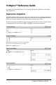
TI-Nspire™ Reference Guide This guide lists the templates, functions, commands, and operators available for evaluating math expressions. Expression templates Expression templates give you an easy way to enter math expressions in standard mathematical notation. When you insert a template, it appears on the entry line with small blocks at positions where you can enter elements. A cursor shows which element you can enter.
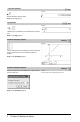
e exponent template u keys Example: Natural exponential e raised to a power Note: See also e^(), page 31. /s key Log template Example: Calculates log to a specified base. For a default of base 10, omit the base. Note: See also log(), page 58. Piecewise template (2-piece) Catalog > Example: Lets you create expressions and conditions for a two-piece piecewise function. To add a piece, click in the template and repeat the template. Note: See also piecewise(), page 73.
System of 2 equations template Catalog > Example: Creates a system of two linear equations. To add a row to an existing system, click in the template and repeat the template. Note: See also system(), page 100. System of N equations template Lets you create a system of N linear equations. Prompts for N. Catalog > Example: See the example for System of equations template (2-equation). Note: See also system(), page 100. Absolute value template Catalog > Example: Note: See also abs(), page 6. dd°mm’ss.
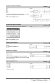
Matrix template (1 x 2) Catalog > Example: . Matrix template (2 x 1) Catalog > Example: Matrix template (m x n) The template appears after you are prompted to specify the number of rows and columns. Catalog > Example: Note: If you create a matrix with a large number of rows and columns, it may take a few moments to appear. Sum template (G) Catalog > Example: Note: See also G() (sumSeq), page 124. Product template (Π) Catalog > Example: Note: See also Π() (prodSeq), page 124.
First derivative template Catalog > Example: The first derivative template can be used to calculate first derivative at a point numerically, using auto differentiation methods. Note: See also d() (derivative), page 123. Second derivative template Catalog > Example: The second derivative template can be used to calculate second derivative at a point numerically, using auto differentiation methods. Note: See also d() (derivative), page 123.
Alphabetical listing Items whose names are not alphabetic (such as +, !, and >) are listed at the end of this section, starting on page 116. Unless otherwise specified, all examples in this section were performed in the default reset mode, and all variables are assumed to be undefined. A abs() Catalog > abs(Value1) ⇒ value abs(List1) ⇒ list abs(Matrix1) ⇒ matrix Returns the absolute value of the argument. Note: See also Absolute value template, page 3.
and Catalog > Integer1 and Integer2 ⇒ integer Compares two real integers bit-by-bit using an and operation. Internally, both integers are converted to signed, 64-bit binary numbers. When corresponding bits are compared, the result is 1 if both bits are 1; otherwise, the result is 0. The returned value represents the bit results, and is displayed according to the Base mode. You can enter the integers in any number base. For a binary or hexadecimal entry, you must use the 0b or 0h prefix, respectively.
Output variable Description stat.SSError Sum of squares of the errors stat.MSError Mean square for the errors stat.sp Pooled standard deviation stat.xbarlist Mean of the input of the lists stat.CLowerList 95% confidence intervals for the mean of each input list stat.CUpperList 95% confidence intervals for the mean of each input list ANOVA2way Catalog > ANOVA2way List1,List2[,List3,…,List10][,levRow] Computes a two-way analysis of variance for comparing the means of two to 10 populations.
Output variable Description stat.PValCol Probability value of the column factor stat.dfCol Degrees of freedom of the column factor stat.SSCol Sum of squares of the column factor stat.MSCol Mean squares for column factor ROW FACTOR Outputs Output variable Description stat.FRow F statistic of the row factor stat.PValRow Probability value of the row factor stat.dfRow Degrees of freedom of the row factor stat.SSRow Sum of squares of the row factor stat.
approx() approx(Value1) Catalog > ⇒ number Returns the evaluation of the argument as an expression containing decimal values, when possible, regardless of the current Auto or Approximate mode. This is equivalent to entering the argument and pressing / ·. approx(List1) ⇒ list approx(Matrix1) ⇒ matrix Returns a list or matrix where each element has been evaluated to a decimal value, when possible.
See coth/(), page 22. arccoth() See csc/(), page 24. arccsc() arccsch() See csch/(), page 24. arcsec() See sec/(), page 88. See sech/(), page 88. arcsech() See sin/(), page 93. arcsin() arcsinh() See sinh/(), page 94. arctan() See tan/(), page 101. See tanh/(), page 102. arctanh() augment() augment(List1, List2) Catalog > ⇒ list Returns a new list that is List2 appended to the end of List1. augment(Matrix1, Matrix2) ⇒ matrix Returns a new matrix that is Matrix2 appended to Matrix1.
avgRC() Catalog > ⇒ expression ⇒ list avgRC(List1, Var [=Value] [, Step]) ⇒ list avgRC(Matrix1, Var [=Value] [, Step]) ⇒ matrix avgRC(Expr1, Var [=Value] [, Step]) avgRC(Expr1, Var [=Value] [, List1]) Returns the forward-difference quotient (average rate of change). Expr1 can be a user-defined function name (see Func). When Value is specified, it overrides any prior variable assignment or any current “with” substitution for the variable. Step is the step value. If Step is omitted, it defaults to 0.001.
4Base2 Catalog > Zero, not the letter O, followed by b or h. 0b binaryNumber 0h hexadecimalNumber A binary number can have up to 64 digits. A hexadecimal number can have up to 16. Without a prefix, Integer1 is treated as decimal (base 10). The result is displayed in binary, regardless of the Base mode. Negative numbers are displayed in “two's complement” form. For example, N1 is displayed as 0hFFFFFFFFFFFFFFFF in Hex base mode 0b111...
4Base16 Catalog > Integer1 4Base16 ⇒ integer Note: You can insert this operator from the computer keyboard by typing @>Base16. Converts Integer1 to a hexadecimal number. Binary or hexadecimal numbers always have a 0b or 0h prefix, respectively. 0b binaryNumber 0h hexadecimalNumber Zero, not the letter O, followed by b or h. A binary number can have up to 64 digits. A hexadecimal number can have up to 16. Without a prefix, Integer1 is treated as decimal (base 10).
centralDiff() Catalog > ⇒ expression centralDiff(Expr1,Var [,Step])|Var=Value ⇒ expression centralDiff(Expr1,Var [=Value][,List]) ⇒ list centralDiff(List1,Var [=Value][,Step]) ⇒ list centralDiff(Matrix1,Var [=Value][,Step]) ⇒ matrix centralDiff(Expr1,Var [=Value][,Step]) Returns the numerical derivative using the central difference quotient formula. When Value is specified, it overrides any prior variable assignment or any current “with” substitution for the variable. Step is the step value.
c2Cdf() Catalog > Cdf(lowBound,upBound,df) ⇒ number if lowBound and upBound are numbers, list if lowBound and upBound are lists chi2Cdf(lowBound,upBound,df) ⇒ number if lowBound and upBound are numbers, list if lowBound and upBound are lists c 2 Computes the c2 distribution probability between lowBound and upBound for the specified degrees of freedom df. For P(X { upBound), set lowBound = 0. For information on the effect of empty elements in a list, see “Empty (void) elements” on page 131.
ClrErr Catalog > ClrErr Clears the error status and sets system variable errCode to zero. For an example of ClrErr, See Example 2 under the Try command, page 105. The Else clause of the Try...Else...EndTry block should use ClrErr or PassErr. If the error is to be processed or ignored, use ClrErr. If what to do with the error is not known, use PassErr to send it to the next error handler. If there are no more pending Try...Else...EndTry error handlers, the error dialog box will be displayed as normal.
completeSquare() completeSquare(ExprOrEqn, Var) Catalog > ⇒ expression or equation completeSquare(ExprOrEqn, Var^Power) equation ⇒ completeSquare(ExprOrEqn, Var1, Var2 [,...]) equation expression or ⇒ completeSquare(ExprOrEqn, {Var1, Var2 [,...
CopyVar Catalog > CopyVar Var1. , Var2. copies all members of the Var1. variable group to the Var2. group, creating Var2. if necessary. Var1. must be the name of an existing variable group, such as the statistics stat.nn results, or variables created using the LibShortcut() function. If Var2. already exists, this command replaces all members that are common to both groups and adds the members that do not already exist. If one or more members of Var2. are locked, all members of Var2. are left unchanged.
μ key cos() cos(squareMatrix1) ⇒ squareMatrix In Radian angle mode: Returns the matrix cosine of squareMatrix1. This is not the same as calculating the cosine of each element. When a scalar function f(A) operates on squareMatrix1 (A), the result is calculated by the algorithm: Compute the eigenvalues (li) and eigenvectors (Vi) of A. squareMatrix1 must be diagonalizable. Also, it cannot have symbolic variables that have not been assigned a value. Form the matrices: Then A = X B X/and f(A) = X f(B) X/.
cosh() Catalog > cosh(Value1) ⇒ value cosh(List1) ⇒ list cosh(Value1) returns the hyperbolic cosine of the argument. cosh(List1) returns a list of the hyperbolic cosines of each element of List1. cosh(squareMatrix1) ⇒ squareMatrix In Radian angle mode: Returns the matrix hyperbolic cosine of squareMatrix1. This is not the same as calculating the hyperbolic cosine of each element. For information about the calculation method, refer to cos(). squareMatrix1 must be diagonalizable.
μ key cot /() cot/(Value1) ⇒ value cot/(List1) ⇒ list In Degree angle mode: Returns the angle whose cotangent is Value1 or returns a list containing the inverse cotangents of each element of List1. In Gradian angle mode: Note: The result is returned as a degree, gradian or radian angle, according to the current angle mode setting. Note: You can insert this function from the keyboard by typing arccot(...).
countif() Catalog > countif(List,Criteria) ⇒ value Returns the accumulated count of all elements in List that meet the specified Criteria. Counts the number of elements equal to 3. Criteria can be: • • A value, expression, or string. For example, 3 counts only those elements in List that simplify to the value 3. A Boolean expression containing the symbol ? as a placeholder for each element. For example, ?<5 counts only those elements in List that are less than 5.
μ key csc() csc(Value1) ⇒ value csc(List1) ⇒ list Returns the cosecant of Value1 or returns a list containing the cosecants of all elements in List1. In Degree angle mode: In Gradian angle mode: In Radian angle mode: μ key csc/() csc /(Value1) ⇒ value csc /(List1) ⇒ list Returns the angle whose cosecant is Value1 or returns a list containing the inverse cosecants of each element of List1.
CubicReg Catalog > CubicReg X, Y[, [Freq] [, Category, Include]] Computes the cubic polynomial regression y = a·x3+b· x2+c·x+d on lists X and Y with frequency Freq. A summary of results is stored in the stat.results variable. (See page 97.) All the lists must have equal dimension except for Include. X and Y are lists of independent and dependent variables. Freq is an optional list of frequency values. Each element in Freq specifies the frequency of occurrence for each corresponding X and Y data point.
Cycle Catalog > Cycle Transfers control immediately to the next iteration of the current loop (For, While, or Loop). Function listing that sums the integers from 1 to 100 skipping 50. Cycle is not allowed outside the three looping structures (For, While, or Loop). Note for entering the example: In the Calculator application on the handheld, you can enter multi-line definitions by pressing @ · instead of at the end of each line. On the computer keyboard, hold down Alt and press Enter.
4DD Expr1 4DD ⇒ value List1 4DD ⇒ list Matrix1 4DD ⇒ matrix Catalog > In Degree angle mode: Note: You can insert this operator from the computer keyboard by typing @>DD. Returns the decimal equivalent of the argument expressed in degrees. The argument is a number, list, or matrix that is interpreted by the Angle mode setting in gradians, radians or degrees.
Define Catalog > Define Function(Param1, Param2, ...) = Func Block EndFunc Define Program(Param1, Param2, ...) = Prgm Block EndPrgm In this form, the user-defined function or program can execute a block of multiple statements. Block can be either a single statement or a series of statements on separate lines. Block also can include expressions and instructions (such as If, Then, Else, and For).
See @List(), page 55. deltaList() DelVar Catalog > DelVar Var1[, Var2] [, Var3] ... DelVar Var. Deletes the specified variable or variable group from memory. If one or more of the variables are locked, this command displays an error message and deletes only the unlocked variables. See unLock, page 109. DelVar Var. deletes all members of the Var. variable group (such as the statistics stat.nn results or variables created using the LibShortcut() function). The dot (.
diag() Catalog > diag(List) ⇒ matrix diag(rowMatrix) ⇒ matrix diag(columnMatrix) ⇒ matrix Returns a matrix with the values in the argument list or matrix in its main diagonal. diag(squareMatrix) ⇒ rowMatrix Returns a row matrix containing the elements from the main diagonal of squareMatrix. squareMatrix must be square. dim() Catalog > dim(List) ⇒ integer Returns the dimension of List. dim(Matrix) ⇒ list Returns the dimensions of matrix as a two-element list {rows, columns}.
4DMS Catalog > Value 4DMS List 4DMS Matrix 4DMS In Degree angle mode: Note: You can insert this operator from the computer keyboard by typing @>DMS. Interprets the argument as an angle and displays the equivalent DMS (DDDDDD¡MM'SS.ss'') number. See ¡, ', '' on page 127 for DMS (degree, minutes, seconds) format. Note: 4DMS will convert from radians to degrees when used in radian mode. If the input is followed by a degree symbol ¡ , no conversion will occur.
eff() Catalog > eff(nominalRate,CpY) ⇒ value Financial function that converts the nominal interest rate nominalRate to an annual effective rate, given CpY as the number of compounding periods per year. nominalRate must be a real number, and CpY must be a real number > 0. Note: See also nom(), page 68.
ElseIf Catalog > If BooleanExpr1 Then Block1 ElseIf BooleanExpr2 Then Block2 © ElseIf BooleanExprN Then BlockN EndIf © Note for entering the example: In the Calculator application on the handheld, you can enter multi-line definitions by pressing @ · instead of at the end of each line. On the computer keyboard, hold down Alt and press Enter. EndFor EndFunc EndIf See For, page 38. See Func, page 40. See If, page 45. EndLoop See Loop, page 60. EndPrgm See Prgm, page 76.
euler() Catalog > euler(Expr, Var, depVar, {Var0, VarMax}, depVar0, VarStep [, eulerStep]) ⇒ matrix euler(SystemOfExpr, Var, ListOfDepVars, {Var0, VarMax}, ListOfDepVars0, VarStep [, eulerStep]) ⇒ matrix euler(ListOfExpr, Var, ListOfDepVars, {Var0, VarMax}, ListOfDepVars0, VarStep [, eulerStep]) ⇒ matrix Differential equation: y'=0.
u key exp() exp(Value1) ⇒ value Returns e raised to the Value1 power. Note: See also e exponent template, page 2. You can enter a complex number in rei q polar form. However, use this form in Radian angle mode only; it causes a Domain error in Degree or Gradian angle mode. exp(List1) ⇒ list Returns e raised to the power of each element in List1. exp(squareMatrix1) ⇒ squareMatrix Returns the matrix exponential of squareMatrix1.
Output variable Description stat.Resid Residuals associated with the exponential model stat.ResidTrans Residuals associated with linear fit of transformed data stat.XReg List of data points in the modified X List actually used in the regression based on restrictions of Freq, Category List, and Include Categories stat.YReg List of data points in the modified Y List actually used in the regression based on restrictions of Freq, Category List, and Include Categories stat.
Fill Catalog > Fill Value, listVar ⇒ list Replaces each element in variable listVar with Value. listVar must already exist. FiveNumSummary Catalog > FiveNumSummary X[,[Freq][,Category,Include]] Provides an abbreviated version of the 1-variable statistics on list X. A summary of results is stored in the stat.results variable. (See page 97.) X represents a list containing the data. Freq is an optional list of frequency values.
For Catalog > For Var, Low, High [, Step] Block EndFor Executes the statements in Block iteratively for each value of Var, from Low to High, in increments of Step. Var must not be a system variable. Step can be positive or negative. The default value is 1. Block can be either a single statement or a series of statements separated with the “:” character.
freqTable4list() Catalog > freqTable4list(List1, freqIntegerList) ⇒ list Returns a list containing the elements from List1 expanded according to the frequencies in freqIntegerList. This function can be used for building a frequency table for the Data & Statistics application. List1 can be any valid list. freqIntegerList must have the same dimension as List1 and must contain non-negative integer elements only.
Output variable Description stat.F Calculated F statistic for the data sequence stat.PVal Smallest level of significance at which the null hypothesis can be rejected stat.dfNumer numerator degrees of freedom = n1-1 stat.dfDenom denominator degrees of freedom = n2-1 stat.sx1, stat.sx2 Sample standard deviations of the data sequences in List 1 and List 2 stat.x1_bar stat.x2_bar Sample means of the data sequences in List 1 and List 2 stat.n1, stat.
geomCdf() Catalog > geomCdf(p,lowBound,upBound) ⇒ number if lowBound and upBound are numbers, list if lowBound and upBound are lists geomCdf(p,upBound) for P(1{X{upBound) upBound is a number, list if upBound is a list ⇒ number if Computes a cumulative geometric probability from lowBound to upBound with the specified probability of success p. For P(X { upBound), set lowBound = 1.
getLockInfo() getLockInfo(Var) Catalog > ⇒ value Returns the current locked/unlocked state of variable Var. value =0: Var is unlocked or does not exist. value =1: Var is locked and cannot be modified or deleted. See Lock, page 57, and unLock, page 109. getMode() Catalog > getMode(ModeNameInteger) getMode(0) ⇒ value ⇒ list getMode(ModeNameInteger) returns a value representing the current setting of the ModeNameInteger mode. getMode(0) returns a list containing number pairs.
getNum() Catalog > getNum(Fraction1) ⇒ value Transforms the argument into an expression having a reduced common denominator, and then returns its numerator. getType() getType(var) Catalog > ⇒ string Returns a string that indicates the data type of variable var. If var has not been defined, returns the string "NONE".
getVarInfo() Catalog > Note the example to the left, in which the result of getVarInfo() is assigned to variable vs. Attempting to display row 2 or row 3 of vs returns an “Invalid list or matrix” error because at least one of elements in those rows (variable b, for example) revaluates to a matrix. This error could also occur when using Ans to reevaluate a getVarInfo() result.
I identity() identity(Integer) Catalog > ⇒ matrix Returns the identity matrix with a dimension of Integer. Integer must be a positive integer. If Catalog > If BooleanExpr Statement If BooleanExpr Then Block EndIf If BooleanExpr evaluates to true, executes the single statement Statement or the block of statements Block before continuing execution. If BooleanExpr evaluates to false, continues execution without executing the statement or block of statements.
If Catalog > If BooleanExpr1 Then Block1 ElseIf BooleanExpr2 Then Block2 © ElseIf BooleanExprN Then BlockN EndIf Allows for branching. If BooleanExpr1 evaluates to true, executes Block1. If BooleanExpr1 evaluates to false, evaluates BooleanExpr2, and so on.
imag() imag(Matrix1) Catalog > ⇒ matrix Returns a matrix of the imaginary parts of the elements. Indirection See #(), page 126. inString() inString(srcString, subString[, Start]) Catalog > ⇒ integer Returns the character position in string srcString at which the first occurrence of string subString begins. Start, if included, specifies the character position within srcString where the search begins. Default = 1 (the first character of srcString).
interpolate() interpolate(xValue, xList, yList, yPrimeList) Catalog > ⇒ list This function does the following: Differential equation: y'=-3·y+6·t+5 and y(0)=5 Given xList, yList=f(xList), and yPrimeList=f'(xList) for some unknown function f, a cubic interpolant is used to approximate the function f at xValue. It is assumed that xList is a list of monotonically increasing or decreasing numbers, but this function may return a value even when it is not.
iPart() Catalog > iPart(Number) ⇒ integer iPart(List1) ⇒ list iPart(Matrix1) ⇒ matrix Returns the integer part of the argument. For lists and matrices, returns the integer part of each element. The argument can be a real or a complex number. irr() Catalog > irr(CF0,CFList [,CFFreq]) ⇒ value Financial function that calculates internal rate of return of an investment. CF0 is the initial cash flow at time 0; it must be a real number. CFList is a list of cash flow amounts after the initial cash flow CF0.
L Lbl Catalog > Lbl labelName Defines a label with the name labelName within a function. You can use a Goto labelName instruction to transfer control to the instruction immediately following the label. labelName must meet the same naming requirements as a variable name. Note for entering the example: In the Calculator application on the handheld, you can enter multi-line definitions by pressing @ · at the end of each line. On the computer keyboard, instead of hold down Alt and press Enter.
libShortcut() Catalog > libShortcut(LibNameString, ShortcutNameString [, LibPrivFlag]) ⇒ list of variables Creates a variable group in the current problem that contains references to all the objects in the specified library document libNameString. Also adds the group members to the Variables menu. You can then refer to each object using its ShortcutNameString.
LinRegMx Catalog > LinRegMx X,Y[,[Freq][,Category,Include]] Computes the linear regression y = m·x+b on lists X and Y with frequency Freq. A summary of results is stored in the stat.results variable. (See page 97.) All the lists must have equal dimension except for Include. X and Y are lists of independent and dependent variables. Freq is an optional list of frequency values. Each element in Freq specifies the frequency of occurrence for each corresponding X and Y data point. The default value is 1.
Output variable Description stat.RegEqn Regression Equation: a+b·x stat.a, stat.b Regression coefficients stat.df Degrees of freedom stat.r2 Coefficient of determination stat.r Correlation coefficient stat.Resid Residuals from the regression For Slope type only Output variable Description [stat.CLower, stat.CUpper] Confidence interval for the slope stat.ME Confidence interval margin of error stat.SESlope Standard error of slope stat.
LinRegtTest Catalog > LinRegtTest X,Y[,Freq[,Hypoth]] Computes a linear regression on the X and Y lists and a t test on the value of slope b and the correlation coefficient r for the equation y=a+bx. It tests the null hypothesis H0:b=0 (equivalently, r=0) against one of three alternative hypotheses. All the lists must have equal dimension. X and Y are lists of independent and dependent variables. Freq is an optional list of frequency values.
linSolve() Catalog > linSolve( SystemOfLinearEqns, Var1, Var2, ...) ⇒ list linSolve(LinearEqn1 and LinearEqn2 and ..., Var1, Var2, ...) ⇒ list linSolve({LinearEqn1, LinearEqn2, ...}, Var1, Var2, ...) ⇒ list linSolve(SystemOfLinearEqns, {Var1, Var2, ...}) ⇒ list linSolve(LinearEqn1 and LinearEqn2 and ..., {Var1, Var2, ...}) ⇒ list linSolve({LinearEqn1, LinearEgn2, ...}, {Var1, Var2, ...}) ⇒ list Returns a list of solutions for the variables Var1, Var2, ...
/u keys ln() ln(squareMatrix1) ⇒ squareMatrix In Radian angle mode and Rectangular complex format: Returns the matrix natural logarithm of squareMatrix1. This is not the same as calculating the natural logarithm of each element. For information about the calculation method, refer to cos() on. squareMatrix1 must be diagonalizable. The result always contains floating-point numbers. To see the entire result, press move the cursor.
Local Catalog > Local Var1[, Var2] [, Var3] ... Declares the specified vars as local variables. Those variables exist only during evaluation of a function and are deleted when the function finishes execution. Note: Local variables save memory because they only exist temporarily. Also, they do not disturb any existing global variable values.
/s keys log() log(Value1[,Value2]) ⇒ value log(List1[,Value2]) ⇒ list Returns the base-Value2 logarithm of the first argument. Note: See also Log template, page 2. For a list, returns the base-Value2 logarithm of the elements. If the second argument is omitted, 10 is used as the base.
Output variable Description stat.RegEqn Regression equation: c/(1+a·e-bx) stat.a, stat.b, stat.c Regression coefficients stat.Resid Residuals from the regression stat.XReg List of data points in the modified X List actually used in the regression based on restrictions of Freq, Category List, and Include Categories stat.YReg List of data points in the modified Y List actually used in the regression based on restrictions of Freq, Category List, and Include Categories stat.
Loop Catalog > Loop Block EndLoop Repeatedly executes the statements in Block. Note that the loop will be executed endlessly, unless a Goto or Exit instruction is executed within Block. Block is a sequence of statements separated with the “:” character. Note for entering the example: In the Calculator application on the handheld, you can enter multi-line definitions by pressing @ · instead of at the end of each line. On the computer keyboard, hold down Alt and press Enter.
max() Catalog > max(Value1, Value2) ⇒ expression max(List1, List2) ⇒ list max(Matrix1, Matrix2) ⇒ matrix Returns the maximum of the two arguments. If the arguments are two lists or matrices, returns a list or matrix containing the maximum value of each pair of corresponding elements. max(List) ⇒ expression Returns the maximum element in list. max(Matrix1) ⇒ matrix Returns a row vector containing the maximum element of each column in Matrix1. Empty (void) elements are ignored.
median() Catalog > median(Matrix1[, freqMatrix]) ⇒ matrix Returns a row vector containing the medians of the columns in Matrix1. Each freqMatrix element counts the number of consecutive occurrences of the corresponding element in Matrix1. Notes: • • All entries in the list or matrix must simplify to numbers. Empty (void) elements in the list or matrix are ignored. For more information on empty elements, see page 131.
mid() Catalog > mid(sourceList, Start [, Count]) ⇒ list Returns Count elements from sourceList, beginning with element number Start. If Count is omitted or is greater than the dimension of sourceList, returns all elements from sourceList, beginning with element number Start. Count must be | 0. If Count = 0, returns an empty list. mid(sourceStringList, Start[, Count]) ⇒ list Returns Count strings from the list of strings sourceStringList, beginning with element number Start.
mod() Catalog > mod(Value1, Value2) ⇒ expression mod(List1, List2) ⇒ list mod(Matrix1, Matrix2) ⇒ matrix Returns the first argument modulo the second argument as defined by the identities: mod(x,0) = x mod(x,y) = x - y floor(x/y) When the second argument is non-zero, the result is periodic in that argument. The result is either zero or has the same sign as the second argument.
MultRegIntervals Catalog > MultRegIntervals Y, X1[,X2[,X3,…[,X10]]],XValList[,CLevel] Computes a predicted y-value, a level C prediction interval for a single observation, and a level C confidence interval for the mean response. A summary of results is stored in the stat.results variable. (See page 97.) All the lists must have equal dimension. For information on the effect of empty elements in a list, see “Empty (void) elements” on page 131. Output variable Description stat.
Output variable Description stat.AdjR2 Adjusted coefficient of multiple determination stat.s Standard deviation of the error stat.DW Durbin-Watson statistic; used to determine whether first-order auto correlation is present in the model stat.dfReg Regression degrees of freedom stat.SSReg Regression sum of squares stat.MSReg Regression mean square stat.dfError Error degrees of freedom stat.SSError Error sum of squares stat.MSError Error mean square stat.bList {b0,b1,...
nDerivative() Catalog > ⇒ value nDerivative(Expr1,Var [,Order]) | Var=Value ⇒ value nDerivative(Expr1,Var=Value[,Order]) Returns the numerical derivative calculated using auto differentiation methods. When Value is specified, it overrides any prior variable assignment or any current “with” substitution for the variable. If the variable Var does not contain a numeric value, you must provide Value. Order of the derivative must be 1 or 2.
nfMin() Catalog > nfMin(Expr, Var) ⇒ value nfMin(Expr, Var, lowBound) ⇒ value nfMin(Expr, Var, lowBound, upBound) ⇒ value ⇒ value nfMin(Expr, Var) | lowBound
normCdf() Catalog > normCdf(lowBound,upBound[,m[,s]]) ⇒ number if lowBound and upBound are numbers, list if lowBound and upBound are lists Computes the normal distribution probability between lowBound and upBound for the specified m (default=0) and s (default=1). For P(X { upBound), set lowBound = .9E999.
nPr() Catalog > nPr(Matrix1, Matrix2) ⇒ matrix Returns a matrix of permutations based on the corresponding element pairs in the two matrices. The arguments must be the same size matrix. npv() Catalog > npv(InterestRate,CFO,CFList[,CFFreq]) Financial function that calculates net present value; the sum of the present values for the cash inflows and outflows. A positive result for npv indicates a profitable investment.
O OneVar Catalog > OneVar [1,]X[,[Freq][,Category,Include]] OneVar [n,]X1,X2[X3[,…[,X20]]] Calculates 1-variable statistics on up to 20 lists. A summary of results is stored in the stat.results variable. (See page 97.) All the lists must have equal dimension except for Include. Freq is an optional list of frequency values. Each element in Freq specifies the frequency of occurrence for each corresponding X and Y data point. The default value is 1. All elements must be integers | 0.
or Catalog > BooleanExpr1 or BooleanExpr2 ⇒ Boolean expression Returns true or false or a simplified form of the original entry. Returns true if either or both expressions simplify to true. Returns false only if both expressions evaluate to false. Note: See xor. Note for entering the example: In the Calculator application on the handheld, you can enter multi-line definitions by pressing @ · at the end of each line. On the computer keyboard, instead of hold down Alt and press Enter.
P4Ry() Catalog > P4Ry(rValue, qValue) ⇒ value P4Ry(rList, qList) ⇒ list P4Ry(rMatrix, qMatrix) ⇒ matrix In Radian angle mode: Returns the equivalent y-coordinate of the (r, q) pair. Note: The q argument is interpreted as either a degree, radian or gradian angle, according to the current angle mode.¡R Note: You can insert this function from the computer keyboard by typing P@>Ry(...). PassErr Catalog > For an example of PassErr, See Example 2 under the Try command, page 105.
4Polar Catalog > Vector 4Polar Note: You can insert this operator from the computer keyboard by typing @>Polar. Displays vector in polar form [r ±q]. The vector must be of dimension 2 and can be a row or a column. Note: 4Polar is a display-format instruction, not a conversion function. You can use it only at the end of an entry line, and it does not update ans. Note: See also 4Rect, page 81. complexValue 4Polar In Radian angle mode: Displays complexVector in polar form.
PowerReg Catalog > PowerReg X,Y [, Freq] [, Category, Include]] Computes the power regression y = (a·(x)b) on lists X and Y with frequency Freq. A summary of results is stored in the stat.results variable. (See page 97.) All the lists must have equal dimension except for Include. X and Y are lists of independent and dependent variables. Freq is an optional list of frequency values. Each element in Freq specifies the frequency of occurrence for each corresponding X and Y data point.
Prgm Catalog > Calculate GCD and display intermediate results. Prgm Block EndPrgm Template for creating a user-defined program. Must be used with the Define, Define LibPub, or Define LibPriv command. Block can be a single statement, a series of statements separated with the “:” character, or a series of statements on separate lines. Note for entering the example: In the Calculator application on the handheld, you can enter multi-line definitions by pressing @ · instead of at the end of each line.
propFrac() Catalog > propFrac(Value1[, Var]) ⇒ value propFrac(rational_number) returns rational_number as the sum of an integer and a fraction having the same sign and a greater denominator magnitude than numerator magnitude. propFrac(rational_expression,Var) returns the sum of proper ratios and a polynomial with respect to Var. The degree of Var in the denominator exceeds the degree of Var in the numerator in each proper ratio. Similar powers of Var are collected.
QuadReg Catalog > QuadReg X,Y [, Freq] [, Category, Include]] Computes the quadratic polynomial regression y = a·x2+b·x+c on lists X and Y with frequency Freq. A summary of results is stored in the stat.results variable. (See page 97.) All the lists must have equal dimension except for Include. X and Y are lists of independent and dependent variables. Freq is an optional list of frequency values. Each element in Freq specifies the frequency of occurrence for each corresponding X and Y data point.
Output variable Description stat.RegEqn Regression equation: a·x4+b·x3+c· x2+d·x+e stat.a, stat.b, stat.c, stat.d, stat.e Regression coefficients stat.R2 Coefficient of determination stat.Resid Residuals from the regression stat.XReg List of data points in the modified X List actually used in the regression based on restrictions of Freq, Category List, and Include Categories stat.
4Rad Catalog > Value14Rad ⇒ value In Degree angle mode: Converts the argument to radian angle measure. Note: You can insert this operator from the computer keyboard by typing @>Rad. In Gradian angle mode: rand() Catalog > rand() ⇒ expression rand(#Trials) ⇒ list Sets the random-number seed. rand() returns a random value between 0 and 1. rand(#Trials) returns a list containing #Trials random values between 0 and 1.
randPoly() Catalog > randPoly(Var, Order) ⇒ expression Returns a polynomial in Var of the specified Order. The coefficients are random integers in the range L9 through 9. The leading coefficient will not be zero. Order must be 0–99. randSamp() Catalog > randSamp(List,#Trials[,noRepl]) ⇒ list Returns a list containing a random sample of #Trials trials from List with an option for sample replacement (noRepl=0), or no sample replacement (noRepl=1). The default is with sample replacement.
4Rect Catalog > complexValue 4Rect In Radian angle mode: Displays complexValue in rectangular form a+bi. The complexValue can have any complex form. However, an reiq entry causes an error in Degree angle mode. Note: You must use parentheses for an (r±q) polar entry. In Gradian angle mode: In Degree angle mode: Note: To type ±, select it from the symbol list in the Catalog. ref() Catalog > ref( Matrix1[, Tol]) ⇒ matrix Returns the row echelon form of Matrix1.
remain() Catalog > remain(Value1, Value2) ⇒ value remain(List1, List2) ⇒ list remain(Matrix1, Matrix2) ⇒ matrix Returns the remainder of the first argument with respect to the second argument as defined by the identities: remain(x,0) x remain(x,y) xNy·iPart(x/y) As a consequence, note that remain(Nx,y) Nremain(x,y). The result is either zero or it has the same sign as the first argument. Note: See also mod(), page 64.
RequestStr Catalog > RequestStr promptString, var [, DispFlag] Define a program: Define requestStr_demo()=Prgm Programming command: Operates identically to the first syntax of the RequestStr “Your name:”,name,0 Request command, except that the user’s response is always Disp “Response has “,dim(name),” characters.” interpreted as a string.
rk23() Catalog > rk23(Expr, Var, depVar, {Var0, VarMax}, depVar0, VarStep [, diftol]) ⇒ matrix rk23(SystemOfExpr, Var, ListOfDepVars, {Var0, VarMax}, ListOfDepVars0, VarStep [, diftol]) ⇒ matrix rk23(ListOfExpr, Var, ListOfDepVars, {Var0, VarMax}, ListOfDepVars0, VarStep [, diftol]) ⇒ matrix Differential equation: y'=0.001*y*(100-y) and y(0)=10 Uses the Runge-Kutta method to solve the system d depVar --------------------- = Expr(Var, depVar) d Var To see the entire result, press move the cursor.
rotate() Catalog > If #ofRotations is positive, the rotation is to the left. If #ofRotations is negative, the rotation is to the right. The default is L1 (rotate right one bit). In Hex base mode: For example, in a right rotation: Each bit rotates right. 0b00000000000001111010110000110101 Important: To enter a binary or hexadecimal number, always use the 0b or 0h prefix (zero, not the letter O). Rightmost bit rotates to leftmost.
rowDim() Catalog > rowDim( Matrix) ⇒ expression Returns the number of rows in Matrix. Note: See also colDim(), page 17. rowNorm() rowNorm( Matrix) Catalog > ⇒ expression Returns the maximum of the sums of the absolute values of the elements in the rows in Matrix. Note: All matrix elements must simplify to numbers. See also colNorm(), page 17. rowSwap() Catalog > rowSwap( Matrix1, rIndex1, rIndex2) ⇒ matrix Returns Matrix1 with rows rIndex1 and rIndex2 exchanged.
S μ key sec() sec(Value1) ⇒ value sec(List1) ⇒ list In Degree angle mode: Returns the secant of Value1 or returns a list containing the secants of all elements in List1. Note: The argument is interpreted as a degree, gradian or radian angle, according to the current angle mode setting. You can use ¡, G, or R to override the angle mode temporarily.
seq() Catalog > seq(Expr, Var, Low, High[, Step]) ⇒ list Increments Var from Low through High by an increment of Step, evaluates Expr, and returns the results as a list. The original contents of Var are still there after seq() is completed. The default value for Step = 1.
seqn() Catalog > Generate the first 6 terms of the sequence u(n) = u(n-1)/2, with u(1)=2. seqn(Expr(u, n [, ListOfInitTerms[, nMax [, CeilingValue]]]) ⇒ list Generates a list of terms for a sequence u(n)=Expr(u, n) as follows: Increments n from 1 through nMax by 1, evaluates u(n) for corresponding values of n using the Expr(u, n) formula and ListOfInitTerms, and returns the results as a list.
Mode Name Mode Integer Setting Integers Exponential Format 3 1=Normal, 2=Scientific, 3=Engineering Real or Complex 4 1=Real, 2=Rectangular, 3=Polar Auto or Approx. 5 1=Auto, 2=Approximate Vector Format 6 1=Rectangular, 2=Cylindrical, 3=Spherical Base 7 1=Decimal, 2=Hex, 3=Binary shift() Catalog > shift(Integer1[,#ofShifts]) ⇒ integer In Bin base mode: Shifts the bits in a binary integer.
sign() Catalog > sign(Value1) ⇒ value sign(List1) ⇒ list sign(Matrix1) ⇒ matrix For real and complex Value1, returns Value1 / abs(Value1) when Value1 ƒ 0. If complex format mode is Real: Returns 1 if Value1 is positive. Returns L1 if Value1 is negative. sign(0) returns „1 if the complex format mode is Real; otherwise, it returns itself. sign(0) represents the unit circle in the complex domain. For a list or matrix, returns the signs of all the elements.
μ key sin() sin(Value1) ⇒ value sin(List1) ⇒ list In Degree angle mode: sin(Value1) returns the sine of the argument. sin(List1) returns a list of the sines of all elements in List1. Note: The argument is interpreted as a degree, gradian or radian angle, according to the current angle mode. You can use ¡,G, or R to override the angle mode setting temporarily.
sinh() Catalog > sinh(Numver1) ⇒ value sinh(List1) ⇒ list sinh (Value1) returns the hyperbolic sine of the argument. sinh (List1) returns a list of the hyperbolic sines of each element of List1. sinh(squareMatrix1) ⇒ squareMatrix In Radian angle mode: Returns the matrix hyperbolic sine of squareMatrix1. This is not the same as calculating the hyperbolic sine of each element. For information about the calculation method, refer to cos(). squareMatrix1 must be diagonalizable.
SinReg Catalog > SinReg X, Y [ , [Iterations] ,[ Period] [, Category, Include] ] Computes the sinusoidal regression on lists X and Y. A summary of results is stored in the stat.results variable. (See page 97.) All the lists must have equal dimension except for Include. X and Y are lists of independent and dependent variables. Iterations is a value that specifies the maximum number of times (1 through 16) a solution will be attempted. If omitted, 8 is used.
SortD Catalog > SortD List1[, List2] [, List3] ... SortD Vector1[,Vector2] [,Vector3] ... Identical to SortA, except SortD sorts the elements in descending order. Empty (void) elements within the first argument move to the bottom. For more information on empty elements, see page 131. 4Sphere Catalog > Vector 4Sphere Note: You can insert this operator from the computer keyboard by typing @>Sphere. Displays the row or column vector in spherical form [r ±q ±f].
stat.results Catalog > stat.results Displays results from a statistics calculation. The results are displayed as a set of name-value pairs. The specific names shown are dependent on the most recently evaluated statistics function or command. You can copy a name or value and paste it into other locations. Note: Avoid defining variables that use the same names as those used for statistical analysis. In some cases, an error condition could occur.
stat.values Catalog > stat.values See the stat.results example. Displays a matrix of the values calculated for the most recently evaluated statistics function or command. Unlike stat.results, stat.values omits the names associated with the values. You can copy a value and paste it into other locations. stDevPop() stDevPop(List[, freqList]) Catalog > ⇒ expression In Radian angle and auto modes: Returns the population standard deviation of the elements in List.
Stop Catalog > Stop Programming command: Terminates the program. Stop is not allowed in functions. Note for entering the example: In the Calculator application on the handheld, you can enter multi-line definitions by pressing @ · at the end of each line. On the computer keyboard, instead of hold down Alt and press Enter. See & (store), page 129. Store string() string(Expr) Catalog > ⇒ string Simplifies Expr and returns the result as a character string.
sum() Catalog > sum(Matrix1[, Start[, End]]) ⇒ matrix Returns a row vector containing the sums of all elements in the columns in Matrix1. Start and End are optional. They specify a range of rows. Any void argument produces a void result. Empty (void) elements in Matrix1 are ignored. For more information on empty elements, see page 131. sumIf() Catalog > sumIf(List,Criteria[, SumList]) ⇒ value Returns the accumulated sum of all elements in List that meet the specified Criteria.
μ key tan() tan(Value1) ⇒ value tan(List1) ⇒ list In Degree angle mode: tan(Value1) returns the tangent of the argument. tan(List1) returns a list of the tangents of all elements in List1. Note: The argument is interpreted as a degree, gradian or radian angle, according to the current angle mode. You can use ¡, G or R to override the angle mode setting temporarily.
tan/() μ key tan/(squareMatrix1) ⇒ squareMatrix In Radian angle mode: Returns the matrix inverse tangent of squareMatrix1. This is not the same as calculating the inverse tangent of each element. For information about the calculation method, refer to cos(). squareMatrix1 must be diagonalizable. The result always contains floating-point numbers. tanh() Catalog > tanh(Value1) ⇒ value tanh(List1) ⇒ list tanh(Value1) returns the hyperbolic tangent of the argument.
tCdf() Catalog > tCdf(lowBound,upBound,df) ⇒ number if lowBound and upBound are numbers, list if lowBound and upBound are lists Computes the Student-t distribution probability between lowBound and upBound for the specified degrees of freedom df. For P(X { upBound), set lowBound = .9E999. Text Catalog > Text promptString [, DispFlag] Programming command: Pauses the program and displays the character string promptString in a dialog box. When the user selects OK, program execution continues.
Output variable Description stat.n Length of the data sequence with sample mean tInterval_2Samp Catalog > tInterval_2Samp List1,List2[,Freq1[,Freq2[,CLevel[,Pooled]]]] (Data list input) tInterval_2Samp v1,sx1,n1,v2,sx2,n2[,CLevel[,Pooled]] (Summary stats input) Computes a two-sample t confidence interval. A summary of results is stored in the stat.results variable. (See page 97.) Pooled=1 pools variances; Pooled=0 does not pool variances.
Try Catalog > Try block1 Else block2 EndTry Executes block1 unless an error occurs. Program execution transfers to block2 if an error occurs in block1. System variable errCode contains the error code to allow the program to perform error recovery. For a list of error codes, see “Error codes and messages,” page 137. block1 and block2 can be either a single statement or a series of statements separated with the “:” character.
Output variable Description stat.t (x N m0) / (stdev / sqrt(n)) stat.PVal Smallest level of significance at which the null hypothesis can be rejected stat.df Degrees of freedom stat.x Sample mean of the data sequence in List stat.sx Sample standard deviation of the data sequence stat.
tvmI() Catalog > tvmI(N,PV,Pmt,FV,[PpY],[CpY],[PmtAt]) ⇒ value Financial function that calculates the interest rate per year. Note: Arguments used in the TVM functions are described in the table of TVM arguments, page 107. See also amortTbl(), page 6. tvmN() Catalog > tvmN(I,PV,Pmt,FV,[PpY],[CpY],[PmtAt]) ⇒ value Financial function that calculates the number of payment periods. Note: Arguments used in the TVM functions are described in the table of TVM arguments, page 107.
TwoVar Catalog > TwoVar X, Y[, [Freq] [, Category, Include]] Calculates the TwoVar statistics. A summary of results is stored in the stat.results variable. (See page 97.) All the lists must have equal dimension except for Include. X and Y are lists of independent and dependent variables. Freq is an optional list of frequency values. Each element in Freq specifies the frequency of occurrence for each corresponding X and Y data point. The default value is 1. All elements must be integers | 0.
Output variable Description stat.MedY Median of y stat.Q3Y 3rd Quartile of y stat.MaxY Maximum of y values stat.G(x-v)2 Sum of squares of deviations from the mean of x 2 Sum of squares of deviations from the mean of y stat.G(y-w) U unitV() unitV(Vector1) Catalog > ⇒ vector Returns either a row- or column-unit vector, depending on the form of Vector1. Vector1 must be either a single-row matrix or a single-column matrix. unLock Catalog > unLock Var1[, Var2] [, Var3] ... unLock Var.
varSamp() varSamp(List[, freqList]) Catalog > ⇒ expression Returns the sample variance of List. Each freqList element counts the number of consecutive occurrences of the corresponding element in List. Note: List must contain at least two elements. If an element in either list is empty (void), that element is ignored, and the corresponding element in the other list is also ignored. For more information on empty elements, see page 131.
While Catalog > While Condition Block EndWhile Executes the statements in Block as long as Condition is true. Block can be either a single statement or a sequence of statements separated with the “:” character. Note for entering the example: In the Calculator application on the handheld, you can enter multi-line definitions by pressing @ · instead of at the end of each line. On the computer keyboard, hold down Alt and press Enter. | “With” See (“with”), page 128.
Z zInterval Catalog > zInterval s,List[,Freq[,CLevel]] (Data list input) zInterval s,v,n [,CLevel] (Summary stats input) Computes a z confidence interval. A summary of results is stored in the stat.results variable. (See page 97.) For information on the effect of empty elements in a list, see “Empty (void) elements” on page 131. Output variable Description stat.CLower, stat.CUpper Confidence interval for an unknown population mean stat.
zInterval_2Prop Catalog > zInterval_2Prop x1,n1,x2,n2[,CLevel] Computes a two-proportion z confidence interval. A summary of results is stored in the stat.results variable. (See page 97.) x1 and x2 are non-negative integers. For information on the effect of empty elements in a list, see “Empty (void) elements” on page 131. Output variable Description stat.CLower, stat.CUpper Confidence interval containing confidence level probability of distribution stat.
zTest zTest Catalog > m0,s,List,[Freq[,Hypoth]] (Data list input) zTest m0,s,v,n[,Hypoth] (Summary stats input) Performs a z test with frequency freqlist. A summary of results is stored in the stat.results variable. (See page 97.) Test H0: m = m0, against one of the following: For Ha: m < m0, set Hypoth<0 For Ha: m ƒ m0 (default), set Hypoth=0 For Ha: m > m0, set Hypoth>0 For information on the effect of empty elements in a list, see “Empty (void) elements” on page 131.
zTest_2Prop Catalog > zTest_2Prop x1,n1,x2,n2[,Hypoth] Computes a two-proportion z test. A summary of results is stored in the stat.results variable. (See page 97.) x1 and x2 are non-negative integers. Test H0: p1 = p2, against one of the following: For Ha: p1 > p2, set Hypoth>0 For Ha: p1 ƒ p2 (default), set Hypoth=0 For Ha: p < p0, set Hypoth<0 For information on the effect of empty elements in a list, see “Empty (void) elements” on page 131. Output variable Description stat.
Symbols + key + (add) Value1 + Value2 ⇒ value Returns the sum of the two arguments. List1 + List2 ⇒ list Matrix1 + Matrix2 ⇒ matrix Returns a list (or matrix) containing the sums of corresponding elements in List1 and List2 (or Matrix1 and Matrix2). Dimensions of the arguments must be equal. Value + List1 ⇒ list List1 + Value ⇒ list Returns a list containing the sums of Value and each element in List1.
N(subtract) - key Value N Matrix1 ⇒ matrix Matrix1 N Value ⇒ matrix Value N Matrix1 returns a matrix of Value times the identity matrix minus Matrix1. Matrix1 must be square. Matrix1 N Value returns a matrix of Value times the identity matrix subtracted from Matrix1. Matrix1 must be square. Note: Use .N (dot minus) to subtract an expression from each element. ·(multiply) r key Value1 ·Value2 ⇒ value Returns the product of the two arguments.
à (divide) p key Value à Matrix1 ⇒ matrix Matrix1 à Value ⇒ matrix Returns a matrix containing the quotients of Matrix1àValue. Note: Use . / (dot divide) to divide an expression by each element. ^ (power) l key Value1 ^ Value2 ⇒ value List1 ^ List2 ⇒ list Returns the first argument raised to the power of the second argument. Note: See also Exponent template, page 1. For a list, returns the elements in List1 raised to the power of the corresponding elements in List2.
.+ (dot add) ^+ keys Matrix1 .+ Matrix2 ⇒ matrix Value .+ Matrix1 ⇒ matrix Matrix1 .+ Matrix2 returns a matrix that is the sum of each pair of corresponding elements in Matrix1 and Matrix2. Value .+ Matrix1 returns a matrix that is the sum of Value and each element in Matrix1. .. (dot subt.) ^- keys Matrix1 .N Matrix2 ⇒ matrix Value .NMatrix1 ⇒ matrix Matrix1 .NMatrix2 returns a matrix that is the difference between each pair of corresponding elements in Matrix1 and Matrix2. Value .
L(negate) v key LLValue1 ⇒ value LList1 ⇒ list LMatrix1 ⇒ matrix Returns the negation of the argument. For a list or matrix, returns all the elements negated. If the argument is a binary or hexadecimal integer, the negation gives the two’s complement. In Bin base mode: Important: Zero, not the letter O To see the entire result, press move the cursor.
= key = (equal) Expr1 = Expr2 ⇒ Boolean expression List1 = List2 ⇒ Boolean list Example function that uses math test symbols: =, ƒ, <, {, >, | Matrix1 = Matrix2 ⇒ Boolean matrix Returns true if Expr1 is determined to be equal to Expr2. Returns false if Expr1 is determined to not be equal to Expr2. Anything else returns a simplified form of the equation. For lists and matrices, returns comparisons element by element.
{ (less or equal) Expr1 { Expr2 ⇒ Boolean expression /= keys See “=” (equal) example. List1 { List2 ⇒ Boolean list Matrix1 { Matrix2 ⇒ Boolean matrix Returns true if Expr1 is determined to be less than or equal to Expr2. Returns false if Expr1 is determined to be greater than Expr2. Anything else returns a simplified form of the equation. For lists and matrices, returns comparisons element by element.
d() (derivative) Catalog > d(Expr1, Var [,Order]) | Var=Value d(Expr1, Var [,Order]) d(List1,Var [,Order]) ⇒ value ⇒ value ⇒ list d(Matrix1,Var [,Order]) ⇒ matrix Except when using the first syntax, you must store a numeric value in variable Var before evaluating d(). Refer to the examples. d() can be used for calculating first and second order derivative at a point numerically, using auto differentiation methods. Order, if included, must be=1 or 2. The default is 1.
Π() (prodSeq) Catalog > Π(Expr1, Var, Low, High) ⇒ expression Note: You can insert this function from the keyboard by typing prodSeq(...). Evaluates Expr1 for each value of Var from Low to High, and returns the product of the results. Note: See also Product template (Π), page 4. Π(Expr1, Var, Low, LowN1) ⇒ 1 Π(Expr1, Var, Low, High) ⇒ 1/Π(Expr1, Var, High+1, LowN1) if High < LowN1 The product formulas used are derived from the following reference: Ronald L. Graham, Donald E. Knuth, and Oren Patashnik.
GInt() Catalog > GInt(NPmt1, NPmt2, N, I, PV ,[Pmt], [FV], [PpY], [CpY], [PmtAt], [roundValue]) ⇒ value GInt(NPmt1,NPmt2,amortTable) ⇒ value Amortization function that calculates the sum of the interest during a specified range of payments. NPmt1 and NPmt2 define the start and end boundaries of the payment range. N, I, PV, Pmt, FV, PpY, CpY, and PmtAt are described in the table of TVM arguments, page 107. • • • If you omit Pmt, it defaults to Pmt=tvmPmt(N,I,PV,FV,PpY,CpY,PmtAt).
/k keys # (indirection) # varNameString Refers to the variable whose name is varNameString. This lets you use strings to create variable names from within a function. Creates or refers to the variable xyz . Returns the value of the variable (r) whose name is stored in variable s1. i key E (scientific notation) mantissaEexponent Enters a number in scientific notation. The number is interpreted as mantissa × 10exponent.
¡ (degree) ¹ key Value1¡ ⇒ value List1¡ ⇒ list Matrix1¡ ⇒ matrix In Degree, Gradian or Radian angle mode: This function gives you a way to specify a degree angle while in Gradian or Radian mode. In Radian angle mode: In Radian angle mode, multiplies the argument by p/180. In Degree angle mode, returns the argument unchanged. In Gradian angle mode, multiplies the argument by 10/9. Note: You can insert this symbol from the computer keyboard by typing @d. ¡, ', '' (degree/minute/second) dd¡mm'ss.
10^() Catalog > 10^ (Value1) ⇒ value 10^ (List1) ⇒ list Returns 10 raised to the power of the argument. For a list, returns 10 raised to the power of the elements in List1. 10^(squareMatrix1) ⇒ squareMatrix Returns 10 raised to the power of squareMatrix1. This is not the same as calculating 10 raised to the power of each element. For information about the calculation method, refer to cos(). squareMatrix1 must be diagonalizable. The result always contains floating-point numbers.
& (store) /h key Value & Var List & Var Matrix & Var Expr & Function(Param1,...) List & Function(Param1,...) Matrix & Function(Param1,...) If the variable Var does not exist, creates it and initializes it to Value, List, or Matrix. If the variable Var already exists and is not locked or protected, replaces its contents with Value, List, or Matrix. Note: You can insert this operator from the keyboard by typing =: as a shortcut. For example, type pi/4 =: myvar.
0B keys, 0H keys 0b, 0h 0b binaryNumber 0h hexadecimalNumber In Dec base mode: Denotes a binary or hexadecimal number, respectively. To enter a binary or hex number, you must enter the 0b or 0h prefix regardless of In Bin base mode: the Base mode. Without a prefix, a number is treated as decimal (base 10). Results are displayed according to the Base mode.
Empty (void) elements When analyzing real-world data, you might not always have a complete data set. TI-Nspire™ Software allows empty, or void, data elements so you can proceed with the nearly complete data rather than having to start over or discard the incomplete cases. You can find an example of data involving empty elements in the Lists & Spreadsheet chapter, under “Graphing spreadsheet data.” The delVoid() function lets you remove empty elements from a list.
List arguments containing void elements(continued) In regressions, a void in an X or Y list introduces a void for the corresponding element of the residual. An omitted category in regressions introduces a void for the corresponding element of the residual. A frequency of 0 in regressions introduces a void for the corresponding element of the residual.
Shortcuts for entering math expressions Shortcuts let you enter elements of math expressions by typing instead of using the Catalog or Symbol Palette. For example, to enter the expression ‡6, you can type sqrt(6) on the entry line. When you press ·, the expression sqrt(6) is changed to ‡6. Some shortrcuts are useful from both the handheld and the computer keyboard. Others are useful primarily from the computer keyboard.
To enter this: Type this shortcut: 4 (conversion) @> 4Decimal, 4approxFraction(), and so on. @>Decimal, @>approxFraction(), and so on.
EOS™ (Equation Operating System) hierarchy This section describes the Equation Operating System (EOS™) that is used by the TI-Nspire™ math and science learning technology. Numbers, variables, and functions are entered in a simple, straightforward sequence. EOS™ software evaluates expressions and equations using parenthetical grouping and according to the priorities described below.
Indirection The indirection operator (#) converts a string to a variable or function name. For example, #(“x”&”y”&”z”) creates the variable name xyz. Indirection also allows the creation and modification of variables from inside a program. For example, if 10&r and “r”&s1, then #s1=10. Post operators Post operators are operators that come directly after an argument, such as 5!, 25%, or 60¡15' 45". Arguments followed by a post operator are evaluated at the fourth priority level.
Error codes and messages When an error occurs, its code is assigned to variable errCode. User-defined programs and functions can examine errCode to determine the cause of an error. For an example of using errCode, See Example 2 under the Try command, page 105. Note: Some error conditions apply only to TI-Nspire™ CAS products, and some apply only to TI-Nspire™ products. Error code Description 10 A function did not return a value 20 A test did not resolve to TRUE or FALSE.
Error code Description 230 Dimension A list or matrix index is not valid. For example, if the list {1,2,3,4} is stored in L1, then L1[5] is a dimension error because L1 only contains four elements. 235 Dimension Error. Not enough elements in the lists. 240 Dimension mismatch Two or more arguments must be of the same dimension. For example, [1,2]+[1,2,3] is a dimension mismatch because the matrices contain a different number of elements.
Error code Description 570 Invalid pathname For example, \var is invalid. 575 Invalid polar complex 580 Invalid program reference Programs cannot be referenced within functions or expressions such as 1+p(x) where p is a program. 600 Invalid table 605 Invalid use of units 610 Invalid variable name in a Local statement 620 Invalid variable or function name 630 Invalid variable reference 640 Invalid vector syntax 650 Link transmission A transmission between two units was not completed.
Error code Description 920 Text not found 930 Too few arguments The function or command is missing one or more arguments. 940 Too many arguments The expression or equation contains an excessive number of arguments and cannot be evaluated. 950 Too many subscripts 955 Too many undefined variables 960 Variable is not defined No value is assigned to variable. Use one of the following commands: • sto & • := • Define to assign values to variables.
Error code Description 1150 Argument error The first two arguments must be polynomial expressions in the third argument. If the third argument is omitted, the software attempts to select a default. 1160 Invalid library pathname A pathname must be in the form xxx\yyy, where: • The xxx part can have 1 to 16 characters. • The yyy part can have 1 to 15 characters. See the Library section in the documentation for more details.
Error code Description 1310 Argument error: A function could not be evaluated for one or more of its arguments.
Warning codes and messages You can use the warnCodes() function to store the codes of warnings generated by evaluating an expression. This table lists each numeric warning code and its associated message. For an example of storing warning codes, see warnCodes(), page 110. Warning code Message 10000 Operation might introduce false solutions. 10001 Differentiating an equation may produce a false equation. 10002 Questionable solution 10003 Questionable accuracy 10004 Operation might lose solutions.
144 TI-Nspire™ Reference Guide
Service and Support Texas Instruments Support and Service For general information For more information about TI products and services, contact TI by e-mail or visit the TI Internet address. E-mail inquiries: ti-cares@ti.com Home Page: education.ti.com Service and warranty information For information about the length and terms of the warranty or about product service, refer to the warranty statement enclosed with this product or contact your local Texas Instruments retailer/distributor.
146 Service and Support
Index Symbols A ^, power 118 ^/, reciprocal 128 :=, assign 129 !, factorial 122 .^, dot power 119 .*, dot multiplication 119 .+, dot addition 119 .N, dot subtraction 119 .
B 4Base10, display as decimal integer 13 4Base16, display as hexadecimal 14 4Base2, display as binary 12 binary display, 4Base2 12 indicator, 0b 130 binomCdf( ) 14 binomPdf( ) 14 Boolean and, and 6 exclusive or, xor 111 not, not 69 or, or 72 C c22way 15 c2Cdf( ) 16 c2GOF 16 c2Pdf( ) 16 Cdf( ) 36 ceiling, ceiling( ) 14, 15, 23 ceiling( ), ceiling 14 centralDiff( ) 15 char( ), character string 15 character string, char( ) 15 characters numeric code, ord( ) 72 string, char( ) 15 clear error, ClrErr 17 ClearA
D d ( ), first derivative 123 days between dates, dbd( ) 26 dbd( ), days between dates 26 4DD, display as decimal angle 27 4Decimal, display result as decimal 27 decimal angle display, 4DD 27 integer display, 4Base10 13 Define 27 Define LibPriv 28 Define LibPub 28 Define, define 27 define, Define 27 defining private function or program 28 public function or program 28 definite integral template for 5 degree notation, - 127 degree/minute/second display, 4DMS 31 degree/minute/second notation 127 delete void e
else if, ElseIf 33 else, Else 45 ElseIf, else if 33 empty (void) elements 131 end for, EndFor 38 function, EndFunc 40 if, EndIf 45 loop, EndLoop 60 program, EndPrgm 76 try, EndTry 105 while, EndWhile 111 end function, EndFunc 40 end if, EndIf 45 end loop, EndLoop 60 end while, EndWhile 111 EndTry, end try 105 EndWhile, end while 111 EOS (Equation Operating System) 135 equal, = 121 Equation Operating System (EOS) 135 error codes and messages 137 errors and troubleshooting clear error, ClrErr 17 pass error, P
getLockInfo( ), tests lock status of variable or variable group 42 getMode( ), get mode settings 42 getNum( ), get/return number 43 getType( ), get type of variable 43 getVarInfo( ), get/return variables information 43 go to, Goto 44 Goto, go to 44 4, convert to gradian angle 44 gradian notation, g 126 greater than or equal, | 122 greater than, > 122 greatest common divisor, gcd( ) 40 groups, locking and unlocking 57, 109 groups, testing lock status 42 H hexadecimal display, 4Base16 14 indicator, 0h 130 hy
augment/concatenate, augment( ) 11 cross product, crossP( ) 23 cumulative sum, cumulativeSum( ) 25 difference, @list( ) 55 differences in a list, @list( ) 55 dot product, dotP( ) 31 empty elements in 131 list to matrix, list4mat( ) 55 matrix to list, mat4list( ) 60 maximum, max( ) 61 mid-string, mid( ) 62 minimum, min( ) 63 new, newList( ) 67 product, product( ) 76 sort ascending, SortA 95 sort descending, SortD 96 summation, sum( ) 99, 100 ln( ), natural logarithm 55 LnReg, logarithmic regression 56 local
maximum, max( ) 61 mean, mean( ) 61 mean( ), mean 61 median, median( ) 61 median( ), median 61 medium-medium line regression, MedMed 62 MedMed, medium-medium line regression 62 mid( ), mid-string 62 mid-string, mid( ) 62 min( ), minimum 63 minimum, min( ) 63 minute notation, ' 127 mirr( ), modified internal rate of return 63 mixed fractions, using propFrac(› with 77 mod( ), modulo 64 mode settings, getMode( ) 42 modes setting, setMode( ) 90 modified internal rate of return, mirr( ) 63 modulo, mod( ) 64 mRow
template for 2 piecewise function (N-piece) template for 2 piecewise( ) 73 poissCdf( ) 73 poissPdf( ) 73 4Polar, display as polar vector 74 polar coordinate, R4Pq( ) 79 coordinate, R4Pr( ) 79 vector display, 4Polar 74 polyEval( ), evaluate polynomial 74 polynomials evaluate, polyEval( ) 74 random, randPoly( ) 81 PolyRoots() 74 power of ten, 10^( ) 128 power regression, PowerReg 74, 75, 83, 84, 103 power, ^ 118 PowerReg, power regression 75 Prgm, define program 76 prime number test, isPrime( ) 49 probability
medium-medium line, MedMed 62 MultReg 64 power regression, PowerReg 74, 75, 83, 84, 103 quadratic, QuadReg 78 quartic, QuartReg 78 sinusoidal, SinReg 95 remain( ), remainder 83 remainder, remain( ) 83 remove void elements from list 29 Request 83 RequestStr 84 result values, statistics 98 results, statistics 97 Return, return 84 return, Return 84 right, right( ) 18, 34, 48, 84, 85, 110 right( ), right 84 rk23( ), Runge Kutta function 85 rotate, rotate( ) 85 rotate( ), rotate 85 round, round( ) 86 round( ), r
stdDevPop( ), population standard deviation 98 stdDevSamp( ), sample standard deviation 98 Stop command 99 storing symbol, & 129 string dimension, dim( ) 30 length 30 string( ), expression to string 99 strings append, & 122 character code, ord( ) 72 character string, char( ) 15 expression to string, string( ) 99 format, format( ) 38 formatting 38 indirection, # 126 left, left( ) 50 mid-string, mid( ) 62 right, right( ) 18, 34, 48, 84, 85, 110 rotate, rotate( ) 85 shift, shift( ) 91 string to expression, exp
time value of money, present value 107 tInterval_2Samp, two-sample t confidence interval 104 tInterval, t confidence interval 103 tPdf( ), student-t probability density 104 trace( ) 104 transpose, T 100 Try, error handling command 105 tTest_2Samp, two-sample t test 106 tTest, t test 105 TVM arguments 107 tvmFV( ) 106 tvmI( ) 107 tvmN( ) 107 tvmPmt( ) 107 tvmPV( ) 107 TwoVar, two-variable results 108 two-variable results, TwoVar 108 U unit vector, unitV( ) 109 unitV( ), unit vector 109 unLock, unlock variab
158