Signals and Measurements for Wireless Communications Testing
Table of Contents Introduction . . . . . . . . . . . . . . . . . . . . . . . . . . . . . . . . . .1 Analog Carriers and Modulation 1 Basic Sine Wave Amplitude Modulation (AM) . . . . . . . . . . . . . . .3 2 AM with Adjacent Carriers 3 Multi-Tone Testing . . . . . . . . . . . . . . . . . . . . . . . . . . . . . . 7 4 Frequency Modulation . . . . . . . . . . . . . . . . . . . . . . . . . . . . 9 5 FM with Dual-Tone Modulation . . . . . . . . . . . . . . . . . . . . . . . .
Signals and Measurements for Wireless Communications Testing Introduction One of the most challenging tasks in designing wireless communications products is the development of a rational approach to characterizing and testing components, assemblies, and sub-systems. Baseband modulation and RF signal characteristics are becoming increasingly complex as standards and common sense force more efficient use of the finite electromagnetic spectrum.
Analog Carriers and Modulation 1 Basic Sine Wave Amplitude Modulation (AM) The best introduction to the AWG is to parallel the procedure of generating a carrier with a conventional signal generator. With a signal generator, one simply enters the carrier frequency and the output amplitude, such as 1000 kHz at 0 dBm. With an AWG, one creates a sequence of points to represent the waveform: A sin ωct where A is the peak amplitude and ωc is the frequency. Since a 0 dBm sinusoid has a peak amplitude of 0.
A record length must be selected that has an adequate number of points to reconstruct the desired waveform. The waveform period is 1 ms and there are 1000 carrier cycles in this period. A record length of 20,000 points would allocate 20 points per cycle, which adequately oversamples the ideal waveform. Any sampling system must sample at least twice as fast as the analog bandwidth of the underlying signal (i.e., 1000 kHz).
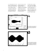
2 AM with Adjacent Carriers A simple addition to the AM signal demonstrates the flexibility of equation-based waveform descriptions. A common task in evaluating receiver performance is to evaluate the effect of adjacent carriers. For the basic AM signal, one can easily add modulated carriers 10 kHz above and below the original signal (Figure 4). One simply adds two copies of the basic AM equation to the original equation.
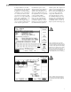
0 -10 Magnitude (dBm) -20 -30 -40 -50 -60 -70 -80 -90 980 985 990 995 1000 1005 Frequency (kHz 8 1010 1015 1020 Figure 6. Spectrum analyzer plot of the 3 carriers. There are 3 kHz AM on the adjacent carriers and 1 kHz AM on the original carrier. Note the low level of close-in spurious components.
Multi-Tone Testing The logical extension of adjacent carrier testing is multi-tone testing. In addition to simulating multiple carriers in a multichannel system, multi-tones can quickly test filter response when a scalar or network analyzer is not available, or they can identify intermodulation products resulting from saturation or nonlinearities in supposedly linear component stages. Traditionally, multi-tone testing requires assembling as many signal generators as desired tones.
The 11 tone equation was then modified so that the last 5 tones (71 through 75 MHz) are inverted. The two different multi-tone results are shown in Figure 9. The scope shows that the rms levels of the two signals are identical, but the peak-topeak values are different. All eleven tones in the original signal added in-phase at t=0. This was not the case with the second signal where 5 of the carriers were inverted at t=0. Thus, the crest factor (peak-torms ratio) of the two signals changed from 4.
Frequency Modulation Frequency modulation introduces control of the phase argument, Φ, in the basic carrier equation: A sin (ωct + Φ ). FM is implemented by varying Φ in direct proportion to the integral of the modulating signal. Thus, for a modulating signal m(t), the FM signal can be written: A sin (ωct + k ∫ m(x) dx ) where k sets the peak frequency deviation.
5 FM with Dual-Tone Modulation While basic single-tone FM is a built-in function of virtually all conventional signal generators, dual-tone FM modulation clearly contrasts the flexibility of the AWG approach. Dual-tone modulation tests can be used to measure intermodulation products in a noise reduction compandor (compressorexpander) in FM receivers such as cordless phones.
Figure 13 shows the demodulated output from an FM receiver with the expander disabled and enabled. The top two traces show the unexpanded two-tone signal and its spectrum as calculated by the TDS 744A FFT function. The lower two traces show the same signals with the expander enabled. The intermodulation products are now significant, with the first order products about 35 dB below the fundamental tones.
6 FM Stereo A final example of conventional analog modulation combines most of the above techniques to simulate the stereo modulation used in broadcast FM. The modulating signal consists of three components, 1) the composite audio which is the sum of the left and right (L+R) channels, 2) the stereo pilot signal which is a 19 kHz tone, and 3) the difference (L-R) signal which amplitude modulates a 38 kHz carrier. These three components are summed together and modulate the carrier using conventional FM.
The resulting 455 kHz signal is mixed up to the broadcast band and inserted into a stereo receiver. The stereo indicator is turned on, and the resulting left and right output signals are captured on the TDS 744A scope (Figure 15). The upper two traces are the right channel (1000 Hz) signal and spectrum. The lower two traces are from the left channel (800 Hz). The stereo encoding was successful with the receiver separating the two tones by over 35 dB. The 38 kHz sub-carrier in FM broad- cast is not unique.
7 Adding Noise to a Carrier Signal — AWG Noise Characteristics Although the removal of noise is a common design goal, a noise source can be an extremely useful test stimulus or signal impairment. The AWG 2041 provides a built-in noise function, but its characteristics are quite different than traditional sources such as noise diodes. An AWG1 noise waveform is actually a calculated series of pseudo-random numbers. There are two key properties of the AWG noise function.
the AWG’s 10 MHz low-pass filter (middle trace). The TDS 744A FFT spectra for the two signals are overlaid below the time domain waveforms. The salient characteristic of the unfiltered noise spectrum is that it rolls off with a (sin x)/x function with the first null at the 32.768 MHz clock frequency and subsequent nulls at multiples of the clock rate. If the goal is to add this noise waveform to the 10.7 MHz FM carrier, then noise density is required only in the vicinity of 10.7 MHz.
The AWG’s graphical waveform editor provides a variety of mathematical operators for existing waveforms. Waveforms can be combined with other waveforms, or a waveform can be squared, scaled, differentiated, integrated, etc. Combining the Noise with the Carrier The signal and noise waveforms are summed using the AWG’s waveform editor (Figure 19). The spectra of the 32K point waveform and the 256K point waveform are overlaid in Figure 20. Recall that the period of the 32K point waveform is 1 ms.
Digital Modulation 8 Digital Phase Modulation — PSK The modulating signals in the foregoing examples have been sinusoidal or continuous waveforms. A simple step to digital modulation is made with a slight variation to sinusoidal modulation. Figure 21 shows one cycle of a sinewave that has been quantized into steps between –0.5 and +0.5. The equation defining these steps is shown in Figure 22.
Figure 22. The equation defining the quantized 1 MHz modulating pattern and its subsequent insertion into the phase argument of the 50 MHz carrier. The modulating pattern shown in Figure 21 is the result of the rounding definition. The record length of 1024 points and a waveform period of 1 µs requires a sampling rate of 1.024 GHz. The resulting carrier frequency is 50 MHz. Since each level represents one of eight states or symbols, 3-bits of data can be transmitted per symbol.
9 Baseband Digital Patterns Before continuing with examples of digital modulation, it is important to establish a method of creating arbitrary test data patterns. Figure 24 shows direct entry of a 28-bit binary pattern. In this case, the 0 or 1 value of each data bit is repeated for 1000 points in the record, which requires a record length of 28,000 points. A binary data pattern requires only one bit of the AWG’s dynamic range.
10 Digital AM — OOK and BPSK The simplest example of digital modulation is to turn the carrier on or off, depending on the state of the modulation data. On-off keying (OOK) can be directly implemented by multiplying a carrier by the 1 or 0 value of the data pattern. This example uses a 10.7 MHz carrier created in a 28,000 point record to match the record length of the data pattern. The AWG sampling rate is 40 MHz so the record period is 700 µs.
11 Digital FM — FSK The modulating data alters the carrier frequency in frequency-shift keying (FSK). A digital modulation index of 0.5 is used in this example; that is, the frequency shift will be 1⁄2 the 40 kbaud data rate or 20 kHz. If the carrier remains centered at 10.7 MHz, this results in the two data frequencies of 10.710 MHz and 10.690 MHz. Figure 28 shows one way to implement binary FSK to take advantage of the AWG’s mathematical precision.
As previously mentioned, the AWG’s two binary marker output signals can be modulated with a data pattern. Figure 30 shows how this can be used as a tool for testing or troubleshooting digital receivers. One marker output is programmed to generate a trigger pulse at the beginning of each 700 µs record (top trace). The second marker is programmed with the 28-bit data pattern (second trace). The two marker signals are generated in real time with the AWG’s main signal output.
12 Quadrature Modulation Multi-level data modulation splits the amplitude, frequency, or phase of the carrier into more than two discrete states. 8-PSK previously demonstrated direct control of the phase Φ in the equation A cos(ωct + Φ); A was constant. The eight symbols were equally spaced points around the polar axes.
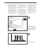
I pattern x carrier Q pattern x carrier Sum Figure 32. Quadrature amplitude modulated (QAM) signal generated by combining an amplitude modulated cosine carrier (upper) and an amplitude modulated sine carrier. There are 16 symbols, so this is 16-QAM. Controller (PC) Oscilloscope (DSO) AWG I In Ch. 1 Out Discrete I Signal Ch. 2 Out Discrete Q Signal DUT Q In I/Q Modulated RF Out RF Generator 26 Figure 33. This block diagram shows the setup for quadrature modulation.
13 Filtering Out Unwanted Sidebands One effect of the edge transitions in digital modulation patterns is a wider than desired occupied spectrum of the transmitted signal. The solution is to filter the baseband digital signal before it modulates the carrier. The two most common filter types for this application are Gaussian and Nyquist filters. Application of the Gaussian filter is illustrated here, though the process for applying any filter type is the same.
The convolution result is 30,000 points long. Note that the impulse response is 2000 points long, which is longer than the 1000 points per data bit. This means that each data bit affects more than the 1000 points that it immediately occupies. Hence, a possible anomaly must be accounted for in the convolution process. The AWG assumes that the data before and after the data pattern is 0. It does not “know” that the data pattern is to repeat over and over.
Figure 36 compares the original and filtered data patterns. The upper two traces are the unfiltered data pattern and its spectrum. The lower two traces are the filtered data pattern and its spectrum. Note how the spectrum of the filtered version rolls off more quickly. The spectrum of a modulated carrier shows the same results. Figure 37 shows the filtered baseband pattern modulating (BPSK) the 10.7 MHz carrier, as in Figure 27. Figure 38 shows the difference in their spectra.
14 Direct Sequence Spread Spectrum The final example of digital modulation spreads the energy in a BPSK signal by amplitude modulating the carrier with a spreading pattern. In the same way that the baseband data pattern spreads the energy of an unmodulated carrier, a spreading pattern further spreads the energy of a modulated carrier. Pseudo-random sequences are generally used as the spreading pattern, with a bit rate or chipping rate that is much higher than the data bit rate.
For More Information on Tektronix Instrumentation Tektronix offers a broad line of signal sources and electronic measurement products for engineering, service, and evaluation requirements in virtually every industry. For detailed information about the Tektronix tools used in developing this booklet, consult the appropriate brochures and data sheets for the respective products: Signal Sources brochure . . . . . . . . . . . . . . . . . . . . . . . . . . .11252 AWG 2005 data sheet . . . . . . . . . . . . . . .
AWG 2000 Series Arbitrary Waveform Generators Tektronix AWG Arbitrary Waveform Generators give the most extensive capabilities for editing waveforms, with 8 or 12 bits of vertical resolution and waveform frequencies to 500 MHz. AWGs contain a high speed, high resolution digital to analog convertor with sophisticated triggering and mode settings, plus up to 4 megabytes of internal memory in which to create and edit waveforms.
TDS 744A Digitizing Oscilloscope The TDS 744A represents the next generation of digitizing scope performance. This versatile general-purpose instrument introduces Tek’s new InstaVu™ acquisition feature and sets a benchmark in waveform capture rate for DSOs. The TDS 744A can display more than 400,000 acquisitions per second—a rate 2,500 times faster than the most advanced DSOs available.
For further information, contact Tektronix: World Wide Web: http://www.tek.