User Manual

Page 18

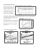
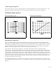
Analysis of the log/log R-C frequency response curve

Some key features:

# the overall characteristic of this network is known as a high-pass filter

# the frequency at which the magnitude falls to 0.707 or -3 dB is known as the "cut-off" or

"corner" frequency of the high-pass filter

# this frequency can be calculated as f(c) = 1/(2πRC), when both the resistance R and capacitance

C are known

# at frequencies well below the cut-off frequency, the plot has the form of a straight line with

gradient +20 dB/decade (in other words, doubling the frequency will double the signal

amplitude) - this characteristic is identical with that of a differentiator network, and gives an output

which is proportional to the rate of change of the input quantity

# at frequencies well above the cut-off frequency, the plot is level at "unity gain" and the output is

directly proportional to the input quantity

# the filter characteristic can be approximated by these two intersecting straight lines, but the

magnitude actually follows an asymptotic curve, with magnitude -3 dB at the cut-off frequency

where the straight lines cross

# the filter characteristic can then be applied to the frequency-domain description of any practical

signal by multiplying the filter transfer characteristic with the spectrum of the input signal, and

deriving a response curve (output) which can in turn be transformed back into a time-domain

signal.

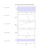
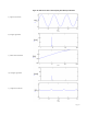
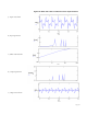
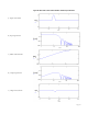
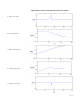
Some practical examples of the effect of this filter characteristic will be shown next. For each signal,

the time-domain description of the "perfect source" (e.g. the waveform which would be seen on an

oscilloscope if the filter characteristic was absent) is given first, followed by its spectrum (obtained by

use of the FFT [Fast Fourier Transform] algorithm supplied in the analysis software), then the filter

characteristic (identical for all examples, but shown to emphasize the effect), then the resulting

output signal spectrum obtained by multiplying the complex input spectrum by the complex filter

characteristic, and finally the corresponding time-domain description obtained by inverse FFT, which

shows the waveform an engineer would expect to observe in reality.

Note: in Figures 15, 16 and 17 the R-C values used to generate the curve were R = 1MΩ

and C = 4.5 nF. In the following plots, the value of C was reduced to 1.5 nF. These

values were chosen somewhat arbitrarily to demonstrate the principle, and so the

scaling on the curves has not been annotated. But the time waveforms can be read in

x units of seconds, and the frequency curves with x units of Hz. The cut-off

frequency for R = 1MΩ and C = 1.5 nF is approximately 106 Hz.