
User's Manual
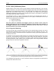
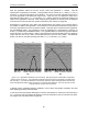
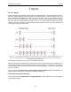
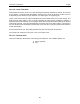
Table Of Contents
- 1 General Overview
- 2 Noggin Components
- 3 Noggin 100 Assembly
- 4 SmartCart Assembly
- 5 SmartTow Assembly
- 6 SmartHandle Assembly (Noggin 500 & 1000 only)
- 7 Rock Noggin Assembly (Noggin 500 & 1000 only)
- 8 Connecting GPS
- 9 Digital Video Logger (DVL)
- 10 Powering Up the System
- 11 Locate & Mark Mode
- 12 Survey & Map Mode
- 12.1 Survey & Map Menu
- 12.2 Data Acquisition
- 12.2.1 Replaying or Overwriting Data
- 12.2.2 Screen Overview
- 12.2.3 Position Information
- 12.2.4 Data Display
- 12.2.5 Section C - Menu
- 12.2.6 Gain
- 12.2.7 Collecting Data using the Odometer
- 12.2.8 Collecting Data in Free Run Mode
- 12.2.9 Collecting Data using the Trigger (or B) Button
- 12.2.10 Noggin Data Screens
- 12.2.11 Calib. (Calibration) Menu
- 12.2.12 Error Messages
- 12.3 Noggin Setup
- 12.4 Noggin File Management
- 12.5 Noggin Utilities
- 13 Troubleshooting
- 14 Care and Maintenance
- Appendix A Noggin Data file Format
- Appendix B Health & Safety Certification
- Appendix C GPR Emissions, Interference and Regulations
- Appendix D Instrument Interference
- Appendix E Safety Around Explosive Devices
- Appendix F Using the PXFER Cable and WinPXFER Software
- F1 Transferring Data to a PC using the PXFER Cable
- F1.1 Connecting the Digital Video Logger to a PC
- F1.2 PXFER Cable Types
- F1.3 Installing and Running the WinPXFER Program
- F1.4 Setting the DVL to the PXFER Cable Type
- F1.5 Transferring Noggin Data Buffer Files
- F1.6 Exporting Nogginplus Data
- F2 Transferring One or More Noggin PCX Files to an External PC using WinPXFER
- Appendix G GPR Glossaries

Noggin 12-Survey & Map Mode
79
12.2.11 Calib. (Calibration) Menu
Noggin systems can be used to scan into many different materials including soil, rock, concrete,
snow, ice and wood. The radio wave emitted by a Noggin system will travel at different velocities
depending on the material being scanned. The depth value (see Section 12.3.1: P.84) and on
Depth Lines (see Section 12.2.4: P.72) are only accurate if the system has been properly
calibrated to determine the velocity of the material being scanned. See Depth on page 84 for
more details about how depth is calculated.
The Calibration function is a tool for determining the velocity of the material being scanned. A
velocity value can be input directly (see Section 12.3.1.2: p.85) or determined in one of two
different ways depending on the situation:
1) Hyperbola matching
2) Target of known depth
Note that unlike the Calibration with Noggin systems (see Section 12.2.11: P.79), the
Noggin
Calibration does NOT automatically update the velocity value in the software. In
the Noggin calibration, once a velocity is determined, the user must enter it into the
System Parameters (see Velocity on page 85).
12.2.11.1Hyperbola Matching
The most accurate way of determining the velocity of the material being scanned is to use the
hyperbola-fitting method because it extracts the velocity using data collected in the area. This
method may not work in all situations because it depends on having a good quality hyperbola (or
inverted U) in the data.
A hyperbola is the characteristic GPR response from a small point target like a pipe, rock or even
a tree root. This phenomenon occurs because radar energy does not radiate as a pencil-thin
beam but more like a 3D cone. Reflections can appear on the record even though the object is
not directly below the radar system. Thus, the radar system “sees” the pipe before and after
going over top of it and forms a hyperbolic reflection.
Figure: 12-3 Hyperbolas in the data result from the conical shape of the GPR energy as it goes into the ground. Tar-
gets, like pipes, are detected as the GPR approaches them (left), passes over them (middle) and after it has passed by
them (right) because the GPR energy propagates both in front and behind the instrument.
If the hyperbola has long tails on it, we can match the shape of the hyperbola and determine the
velocity of the material in the area.