Allen-Bradley Synchronized Axes Control Module (Cat. No.
Important User Information Because of the variety of uses for the products described in this publication, those responsible for the application and use of this control equipment must satisfy themselves that all necessary steps have been taken to assure that each application and use meets all performance and safety requirements, including any applicable laws, regulations, codes and standards.
toc–i System Overview Chapter 1 Chapter Objectives . . . . . . . . . . . . . . . . . . . . . . . . . . . . . . . . . . . What Is the 1746-QS Module? . . . . . . . . . . . . . . . . . . . . . . . . . . . What Is the Hydraulic Configurator . . . . . . . . . . . . . . . . . . . . . . . . What Is an SLC-500 System? . . . . . . . . . . . . . . . . . . . . . . . . . . . . Why Use This System? . . . . . . . . . . . . . . . . . . . . . . . . . . . . . . . . How Does It Work? . . . . . . . . . . . . . . . . . . .
toc–ii Adjusting Command-word Speed and Acceleration Values . . . . . Adjusting Feedforward Parameters . . . . . . . . . . . . . . . . . . . . . . Using Acceleration Feedforwards . . . . . . . . . . . . . . . . . . . . . . . Adjusting P-I-D Gains . . . . . . . . . . . . . . . . . . . . . . . . . . . . . . . . Finding the Value of the Dead Band Eliminator . . . . . . . . . . . . . . . . Saving Parameters . . . . . . . . . . . . . . . . . . . . . . . . . . . . . . . . . . .
Chapter 1 Chapter Objectives This chapter presents a conceptual overview of how you use the 1746-QS module in an application. What Is the 1746-QS Module? The 1746-QS Synchronized Axes Module provides four axes of closed-loop synchronized servo positioning control, and lets you change motion parameters while the axis is moving.
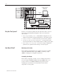
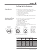
1–2 Hydraulic Configurator Software on PC For Setup and Troubleshooting HYDRAULIC Power Supply 1747-CP3 Cable SYNCHR AXES 1492-ACABLE015Q SLC-500 Processor 1746-QS module Position Input One of Four Identical Motion-control Loops Interface Module (terminal block) 1492-AIFMQS Analog Output "10V dc Axis Motion Why Use This System? Proportional Amplifier Servo-quality Proportional Valve Piston-type Hydraulic Cylinder and Position-monitoring Device Because you can interact quickly and easily with
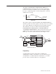
1–3 The MODE, ACCELERATION, DECELERATION, SPEED, and COMMAND VALUE (requested position) are used to generate the profile. You send these command words to the module through the processor’s output image table. You may change them “on-the-fly“ while the axis is moving. Max Speed Speed Accel Ramp Decel Ramp Command Value (Final Position) Time Motion Profile The module compares ACTUAL POSITION with TARGET POSITION to determine position error.
1–4 Ladder logic transfers motion commands to the module and axis status from the module thru the I/O image table. Ladder logic also copies configuration parameters to the module’s M0 file at power up. It also copies configuration parameters (that you enter/change with the Hydraulic Configurator) from the module’s M1 file to processor files.
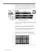
Chapter 2 Setting Up the Hardware Chapter Objectives This chapter helps you install the hardware with these tasks: • • • • • • Connections to LDTs and 4-axis Terminal Block connecting LDTs to the Interface Module (IFM) terminal block minimizing interference from radiated electrical noise connecting outputs to output devices checking out the wiring and grounding setting up the hydraulics regarding the Interface Module (IFM) terminal block and cable We assume that you will use one of the following type
2–2 Typical Connections to the Interface Module (IFM) Terminal Block Pin assignments of the IFM terminal block for I/O, power, shield, and ground connections are as follows: (For example, we show connections for one axis with a Temposonics LDT and power supply.
2–3 Wiring Example We present a 1-axis loop with a differential LDT input. (You must provide power supplies and servo amplifiers.) "15V Power Supply for LDTs (–) (C) (+) 24V Power Supply (+) (–) Axis Loop 1 of 4-axis system Important: The module’s analog outputs require an external amplifier to drive the valve. Belden 8761 Connect cable shields of LDT and drive output to SH terminals on terminal block (to earth GND).
2–4 Important: To minimize the adverse effects of ground loops, you must isolate power supply and signal commons from earth ground as follows: 1. Connect power supply commons to IFM Com terminal (50), and LDT commons to LDT Com terminals of the IFM terminal block. Be sure that they are isolated from earth ground. 2. Connect the cable shield of the servo or proportional amplifier output cable to a zero potential terminal inside the amplifier. 3. Use bond wires that are equal in size to signal wires. 4.
2–5 Checking Out the Wiring and Grounding Repeat this procedure to check out each of the four axis loops connected to the IFM terminal block. ATTENTION: Be sure to remove all power to the SLC processor, LDT, valve and pump beforehand. 1. Disconnect the LDT connector at the head end. 2. Disconnect the connector to the IFM terminal block. 3. Turn ON the power supplies for the LDT and SLC processor, and check the LDT connector and IFM terminal block for: • +15V dc • PS common • –15V dc 4.
2–6 5. Avoid valves with a slow response (less than 60 Hz). Valves with slow response cause the module to overcompensate for disturbances in the motion of the system. Since the system does not respond immediately to the control signal, the module continues to increase the drive signal. By the time the system begins to respond to the error, the control signal has become too large and the system overshoots. The module then attempts to control in the opposite direction, but again overshoots.
Chapter 3 Setting Up Your PC for the Hydraulic Configurator Chapter Objectives This chapter helps you do the following: • Obtain the Hydraulic Configurator from the Internet • Set up communication between your PC and the module Obtaining the Hydraulic Configurator from the Internet You can download the Hydraulic Configurator from our website to your PC. (You can also download ladder logic and transfer it to your SLC processor, but we cover that in chapter 6.
3–2 Setting Up Communication Between PC and Module You must establish communication between Hydraulic Configurator software on your PC and the module. 1. Connect your PC to the module with Allen-Bradley cable (cat. no. 1747-CP3): one end to a serial port on your PC such as COM1, the other end to the 9-pin D-shell connector on the module. Windows ’95 provides a virtual connection to the serial port without any intervention unless that port is already used by another application.
Chapter 4 Tuning an Axis with the Hydraulic Configurator Chapter Objectives We cover these topics: • • • • • • • Before You Begin Before You Begin Finding the Value of the Null Drive Moving the Axis to Set Offset, Scale, Extend and Retract Limits Getting Ready to Tune the Axes Tuning Each Axis Finding the Value of the Dead Band Eliminator Saving Parameters ATTENTION: Great care must be taken to avoid accidents when starting the module for the first time.
4–2 1. 2. 3. 4. 5. 6. 7. 8. Moving the Axis to Set Scale, Offset, Extend, and Retract Limits Turn off the power to the module. Connect the axis drive output to the amplifier. Turn the power back on. Turn on the hydraulics. If the axis drifts, go to step 5. If not, you are done. Go to the next procedure, Moving the Axis. Find the Null Drive value to stop axis drift: a) Estimate a drive output (mV) required to hold zero motion.
4–3 1. 2. 3. 4. 5. Turn off the power to the module. Disconnect the axis drive output to the amplifier. Turn the power back on. Turn on the hydraulics. Move the axis to the first position with the diddle box. It doesn’t matter whether the first position is an extend or retract. 6. In the Scale/Offset Calibration window (from Tools in command bar): a) Enter the desired position value into the Actual Position field for the First Position.
4–4 3. Turn the power back on. 4. Turn on the hydraulics. If the axis drifts, go back to the Null Drive procedure. If not, go to step 5. 5. To move the axis to the first position (either extend or retract). a) Estimate drive output (mV) that would generate a slow safe speed. Enter it into the COMMAND VALUE number field. Note: In open-loop mode, this field sets the module output. In closed-loop mode, this field sets the commanded position. b) Command the module to output that value with the “O“ command.
4–5 Getting Ready to Tune the Axes Once you have set scale, offset, and extend/retract limits in open-loop mode, you can now use the Hydraulic Configurator to tune the axis using closed-loop move commands and axis plots. We suggest that you: 1. Leave un-entered configurations parameters at default, except for: – Auto Stop to 000E0 (hard stop, only for LDT faults) 2. If not done already, initialize the axes with the “P” command. 3.
4–6 2. The Following Error will probably vary as indicated by diverging plots of target and actual speeds during acceleration or deceleration. Target Speed (pink) Actual Speed (dark blue) Following Error 3. To achieve a nearly constant steady-state Following Error, increase the PROPORTIONAL GAIN until the plots of target and actual speeds become parallel during acceleration or deceleration. 4. To minimize the Following Error, use the auto Adjust Feedforward “F” command.
4–7 7. If moving a relatively large mass with a relatively small hydraulic cylinder, first investigate the affect of: a) Integrator Mode selection in the Command-mode word: active always, for accel/decels, in position, or never. b) Integrator Limit selection in the Config word: 20% for a typical hydraulic system, 80% for a difficult system. Also, see step 6 for using INTEGRAL GAIN to help minimize the end-point position error. For additional information on PID Gains, refer to that topic, below.
4–8 Important: When tuning the Feedforward term with command “F”, plot sequential axis moves and compare plots of target position and actual position until the two plots coincide. Another way to adjust these parameters is to set the DIFFERENTIAL GAIN and INTEGRAL GAIN to zero and the PROPORTIONAL GAIN to a small value (between 1 and 5), then make long slow moves in both directions. Adjust the EXT FEEDFORWARD and RET FEEDFORWARD until the axis tracks within 10% in both directions.
4–9 It is usually desirable to have some INTEGRAL GAIN (5 to 50 counts) to help compensate for valve null drift or changes in system dynamics. Some systems may require larger INTEGRAL GAIN, in particular if they are moving a large mass or are nonlinear. Too much INTEGRAL GAIN will cause oscillations. On the other hand, some hydraulic systems do not require INTEGRAL GAIN. DIFFERENTIAL GAIN is used mainly on systems which have a tendency to oscillate.
4–10 6. Back down the value below no motion. Write down this valve. 7. Repeat steps 1-6 with negative values for opposite direction. 8. Determine DEAD BAND ELIMINATOR value. It is the larger of the values from step 6, regardless of sign ("). 9. Enter the value of the DEAD BAND ELIMINATOR in the number field in the Parameter section of the main screen. 10.Transfer the parameter to the module using the “P” Command.
Chapter 5 Using Ladder Logic Chapter Objectives This chapter covers: • Obtaining sample ladder program from the Internet • Configuring your SLC processor, off-line • Using the sample ladder program, RSExampl.
5–2 Using the Sample Ladder Program Consider creating a bit and data address table for your own applicaion.
5–3 Copy Configuration Parameters to the SLC Processor | INITIALIZE GET from QS Module | Enable this rung to copy configuration parameters to the SLC N file | | after you change them with the Hydraulic Configurator. | | | | Set ON to read | | parameters | | after tuning Parameters for Axis 1 | | GET_PARAMETERS CONFIG1 | | B3:0 +COP–––––––––––––––+ | |–––] [–––––––––––––––––––––––––––––––––––––––––+–+COPY FILE +–+–| | 1 | |Source #M1:2.
5–4 Back and Forth Motion with State-machine Logic (Programming for Automatic Operation) This ladder logic example moves axes 1 and 2 back and forth with Go “G” commands. Each move has its own set of motion profile words (mode, accel, decel, speed, and position). The example is a state machine with four automatic states: State: 0 1 2 3 Description: No motion.
5–5 | | | Reset the state machine for all axes if not in auto mode. | | In state 0, the auto mode state machine does not write to the module’s I/O. | | | | Run state | | machine | | example | | AUTO_MODE AXIS1_NEXT_STATE | | B3:0 +FLL–––––––––––––––+ | |–––]/[–––––––––––––––––––––––––––––––––––––––––––––––––––––––+FILE FILL +–| | 14 |Source 0 | | | |Dest #N7:4 | | | |Length 4 | | | +––––––––––––––––––+ | | | | Copy next state to state machine. | | This technique avoids race conditions.
5–6 | AXIS 1 and 2 STATE 2 | | | | Use motion profile words (mode, accel, decel, speed, and command) stored in | | N12:6-11 (axis 1) and N12:18-23 (axis 2). | | Wait for IN-POSITION bit to go high. Then set NEXT STATE to 3. | | | | Oneshot | | AXIS1_STATE storage Bit AXIS1_MODE | | +EQU–––––––––––––––+ B3:1 +COP–––––––––––––––+ | |––+EQUAL +––+–––[OSR]––––––––––––––––––––––+–+COPY FILE +–+–+–| | |Source A N7:0 | | 12 | |Source #N:12.6| | | | | | 3<| | | |Dest #O:2.
5–7 Jogging the Axes In the sample program: – Commands for jogging axis 1 are stored in N12:24-29 (to advance) and N12: 30-35 (to retract). – Jog “pushbutton” addresses are B3:0/3 (advance) and B3:0/4 (retract). When either jog “pushbutton” is pressed: – extend and retract limits are copied into the jog command position words in the N files – the corresponding N file is copied to the output word to the module This provides a target position at the end of travel in each direction.
5–8 | Run State | | Axis 1 Jog Retract Machine Oneshot | | (Jog Pushbutton Example Storage | | + interlocks AUTO_MODE Bit AXIS1_MODE | | B3:0 B3:0 B13:4 +COP–––––––––––––––+ | |–––––––––] [––––––––––––––]/[––––+–––––––––––––––––[OSR]–––+COPY FILE +–+–| | 4 14 | 5 |Source #N12.30| | | | | |Dest #O:2.
5–9 | ATTENTION: When hydraulic system power is lost, your ladder logic is responsible | | for ensuring that valve null and integrator sum do not wind up if the axis is | | out of position. If wind up is allowed, the axis will move unexpectedly when | | hydraulic system is restored.
5–10 Notes: Publication 1746-6.
Chapter 6 Troubleshooting Objectives This chapter: • Describes the module’s LED indicators • Suggests corrective action for typical operating problems Using LED Indicators Use this table to interpret the module’s LED-indicated status. HYDRAULIC RUN/FLT AXES 1 3 2 4 SYNCHR AXES Correcting Typical Problems Problem Condition: Use this table to look up corrective action for typical problems.
6–2 Notes: Publication 1746-6.
Module Specifications Electrical SLC Processor Backplane Power Requirements I/O Chassis Location I/O Image Table Usage Configuration Parameters For use with SLC 5/03 or SLC 5/04 processors 1.
A–2 Module Specifications Environmental Operating Temperature 0°C to 60°C (32°F to 140°F) Storage Temperature –40°C to +85°C (–40°F to +185°F) Relative Humidity 5% to 93% (without condensation) Agency Certification (when marked on product or package) CE marked for all applicable directives Certification Publication 1746-6.
B Appendix Wiring Without the Interface Module Wiring Example We present a 1-axis loop with a differential LDT input. (You must provide power supplies and servo amplifiers.) "15V Power Supply 24V Power Supply (–) (C) (+) (+) (–) Belden 8761 Axis Loop 1 of 4-axis system Belden 8770 Connect cable shields to earth ground. Connect signal commons and PS commons together, isolated from earth ground.
B–2 Wiring Without the Interface Module Minimizing Interference from Radiated Electrical Noise Important: Signals in this type of control system are very susceptible to radiated electrical noise. Minimize interference from radiated electrical noise with correct shielding and grounding as follows: Connect LDT cable shields and drive output cable shields (all shields at one end, only) to earth ground. Keep LDT signal cables far from motors or proportional amplifiers.
Appendix C Using Processor Files This appendix covers these topics: • Transferring Data • M0 and M1 files – for initial configuration • I/O image table – to write commands and read status while running Transferring Data Overview The module communicates with the SLC processor over the I/O backplane. Motion commands and axis status for all four axes are transferred across the backplane in groups of 32, 16-bit words in output image table O:e.0-31 for commands and input image table I:e.0-31 for status.
C–2 Using Processor Files Transferring Motion Commands and Axis Status Motion commands and axis status can be integer or floating-point values. Important: If your application requires position values > 32,767, you must use floating-point values and your ladder logic instructions must: compute floating-point numbers from integer • store values in floating-point (F) files Each of four files contains the 8-word motion command for an axis. The eight words define the axis’ motion profile.
Using Processor Files Axis 4 #Nx:48 Axis 3 #Nx:32 Axis 2 #Nx:16 Axis 1 #Nx:0 Each N file contains 16 words of Configuration Parameters 16-word Files for Axis Configuration Parameters C–3 Module’s M0 File >>> >>> Ladder Logic COPY instructions >>> >>> 16-word Files for Axis Configuration Parameters When commanded, ladder logic copies 16 words of axis configuration parameters from the module’s M1 file to processor N files.
C–4 Using Processor Files Using M0 and M1 Files for Initial Configuration Configuration parameters for M0 and M1 files can be stored in three locations: on PC disk, in SLC-processor N files, and in module FLASH memory. The “P” command activates the parameters (moves them from RAM to control CPU in the module). Disk PC Configuration Parameters P Cmd. N Files SLC Configuration Parameters M0/M1 Files in Module RAM COPY FLASH P Cmd.
Using Processor Files C–5 Bit Map of Configuration Word (e:0, e:16, e:32. e:48) Word Configuration (bit map) ap) Using I/O Image Tables for Commands and Status Bit Description 15-12 Number of LDT recirculations = bit combination. bit 15 = 8 recirculations bit 14 = 4 recirculations bit 13 = 2 recirculations bit 13 = 1 recirculation 11-04 Reserved 03 Simulate mode, used for debugging. = 1 Drive output is set to null, LDT inputs are ignored.
C–6 Using Processor Files Bit Map of Command Mode Word Word Bit 15 Co and Mode Command (Co and word 0)) (Command 14-08 07 06 05-04 03-02 01-00 0= 1= Description plots each move of the axis, overwwriting previous plot disables axis plot to preserve the last plot reserved 0 = disables S Curve 1 = module computes an S-curve target for smoother motion 0 = disables Quick Mode 1 = module ramps up to (max) drive output in open loop, maintains it, then ramps down in closed loop axis limit Synch A/B: Axes
A E applications, of module, 1-4 electrical noise, minimize, 2-3, 2-4, 2-5 axis, connections for control loop, 2-3 getting ready to move, 4-5 jogging, sample program, 5-7 stopping axis motion, 4-10 synchronized motion, 5-9 tuning, 4-1 error, following, 4-6 Sun-Error2, 4-6, 4-8 B benefits, of module, 1-2 bits, 5-2, C-5, C-6 C cables, 4-3 Interface Module to QS module, 2-6 grounding of, 2-3 PC to module, 2-3, 3-2 system, 1-2, 2-3 calibration, set scale and offset, 4-3, 4-4 commands, to module, “K”
I–2 Index L ladder logic (see sample programs) data transfer concepts, C-1 download from Internet, 5-1 processor files, C-1 sample programs, 5-2 words/bits, 5-2 LDT connections to, 2-1, 2-2 identify type in Hydraulic Configurator, 4-1 length/resolution of, A-1 types, 2-1 LED indicators, 6-1 M M0/M1 files, C-3, C-4 I/O configuration in SLC, 5-1 ladder to copy parameters to module, 5-3 N N files, chapter 5, appendix C noise, electrical, 2-3 null drive, finding its value, 4-1 O offset, finding its value,
Allen-Bradley, a Rockwell Automation Business, has been helping its customers improve productivity and quality for more than 90 years. We design, manufacture and support a broad range of automation products worldwide. They include logic processors, power and motion control devices, operator interfaces, sensors and a variety of software. Rockwell is one of the world’s leading technology companies. Worldwide representation.