Overview of This Tutorial - Department of Geosciences

Tutorial: Hyperspectral Signatures and Spectral Resolution
Open GER63 Image
5. From the ENVI main menu bar, select File → Open Image File. A file selection dialog appears.
6. Navigate to envidata\cup_comp and select cupgersb.img. Click Open.
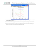
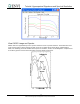
7. To optionally view a color composite that enhances mineralogical differences, select the RGB Color
radio button, select Band 36, Band 42, and Band 50, and click Load RGB.
8. In the Available Bands List, select the Gray Scale radio button, select Band 42, and click Load
Band.
9. From the Display group menu bar, select Tools → Profiles → Z Profile (Spectrum). A Spectral
Profile plot window appears.
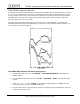
10. From the Display group menu bar, select Tools → Pixel Locator. A Pixel Locator dialog appears.
11. Enter the pixel location (235, 322), a kaolinite feature, and click Apply.
12. Right-click in the Spectral Profile plot window and select Collect Spectra.
13. Enter the following pixel locations and click Apply each time.
Alunite (303, 240)
Buddingtonite (185, 233)
Silica or Opal (289, 253)
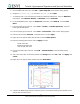
14. From the Spectral Profile menu bar, select Edit → Plot Parameters. A Plot Parameters dialog
appears.
15. The X-Axis radio button is selected by default. Enter Range values from 2.0 to 2.5. Click Apply, then
Cancel.
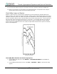
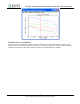
16. Right-click in the Spectral Profile window and select Stack Plots.
17. Compare the GER63 image spectra to the library spectra (in the Spectral Library Plots window) and to
spectra from the other sensors.
13
ENVI Tutorial: Hyperspectral Signatures and Spectral Resolution