Overview of This Tutorial - Department of Geosciences

Tutorial: Hyperspectral Signatures and Spectral Resolution
10
ENVI Tutorial: Hyperspectral Signatures and Spectral Resolution
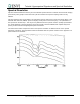
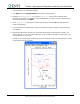
3. Select cupgs_em.txt and click Open. An Input ASCII File dialog appears. Click OK to plot the
kaolinite and alunite spectra in the ENVI Plot Window.
4. Compare these spectra to the USGS library spectra (in the Spectral Library Plots window) and to the
spectra from the other sensors.
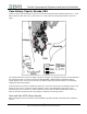
Open GEOSCAN Image
5. From the ENVI main menu bar, select File → Open Image File. A file selection dialog appears.
6. Navigate to envidata\cup_comp and select cupgs_sb.img. Click Open. This file contains
GEOSCAN imagery of Cuprite (collected in 1989), at approximately 60 nm spectral resolution with 44
nm sampling, converted to apparent reflectance using a Flat Field correction in ENVI.
7. To optionally view a color composite that enhances mineralogical differences, select the RGB Color
radio button, select Band 13, Band 15, and Band 18, and click Load RGB.
8. In the Available Bands List, select the Gray Scale radio button, select Band 15, and click Load
Band.
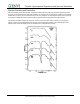
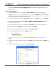
9. From the Display group menu bar, select Tools → Profiles → Z Profile (Spectrum). A Spectral
Profile plot window appears.
10. From the Display group menu bar, select Tools → Pixel Locator. A Pixel Locator dialog appears.
11. Enter the pixel location (275, 761), a kaolinite feature, and click Apply.
12. Right-click in the Spectral Profile plot window and select Collect Spectra.
13. Enter the following pixel locations and click Apply each time.
Alunite (435, 551)
Buddingtonite (168, 475)
Silica or Opal (371, 592)
14. From the Spectral Profile menu bar, select Edit → Plot Parameters. A Plot Parameters dialog
appears.
15. The X-Axis radio button is selected by default. Enter Range values from 2.0 to 2.5. Click Apply, then
Cancel.
16. Right-click in the Spectral Profile window and select Stack Plots.