ENVI Tutorial: Hyperspectral Signatures and Spectral Resolution Table of Contents OVERVIEW OF THIS TUTORIAL ..................................................................................................................... 2 SPECTRAL RESOLUTION ............................................................................................................................. 3 Spectral Modeling and Resolution .....................................................................................................
Tutorial: Hyperspectral Signatures and Spectral Resolution Overview of This Tutorial This tutorial compares the spectral resolution of several different sensors and the effect of resolution on the ability to discriminate and identify materials with distinct spectral signatures.
Tutorial: Hyperspectral Signatures and Spectral Resolution Spectral Resolution Spectral resolution determines the way we see individual spectral features in materials measured from imaging spectrometry. Many people confuse the terms spectral resolution and spectral sampling. These are very different. Spectral resolution refers to the width of an instrument response (band-pass) at half of the band depth, or the full width half maximum (FWHM).
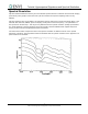
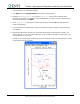
Tutorial: Hyperspectral Signatures and Spectral Resolution Spectral Modeling and Resolution Spectral modeling shows that spectral resolution requirements for imaging spectrometers depend upon the character of the material being measured. Kaolinite, for example (see the plot below), exhibits a characteristic doublet near 2.2 µm at 20 nm resolution.
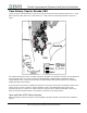
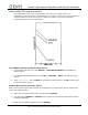
Tutorial: Hyperspectral Signatures and Spectral Resolution Case History: Cuprite, Nevada, USA Cuprite has been used extensively as a test site for remote sensing instrument validation (Abrams et al., 1978; Kahle and Goetz, 1983; Kruse et al., 1990; Hook et al., 1991). Refer to the following alteration map of the region. This tutorial illustrates the effects of spatial and spectral resolution on information extraction from multispectral and hyperspectral data.
Tutorial: Hyperspectral Signatures and Spectral Resolution 1. From the ENVI main menu bar, select Spectral → Spectral Libraries → Spectral Library Viewer. A Spectral Library Input File dialog appears. 2. Click Open and select Spectral Library. A file selection dialog appears. 3. Navigate to envidata\cup_comp and select usgs_em.sli. These spectra represent USGS laboratory measurements for kaolinite, alunite, buddingtonite, and opal, in Cuprite, measured with a Beckman spectrometer. Click Open. 4.
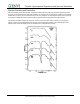
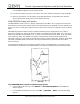
Tutorial: Hyperspectral Signatures and Spectral Resolution View Landsat TM Image and Spectra The following plot shows region of interest (ROI) mean spectra for kaolinite, alunite, and buddingtonite. The small squares indicate the TM band 7 (2.21 µm) center point. The lines indicate the slope from TM band 5 (1.65 µm). The spectra appear very similar, and you cannot effectively discriminate between the three endmembers. View TM Mean Kaolinite and Alunite Image Spectra 1.
Tutorial: Hyperspectral Signatures and Spectral Resolution 7. For easier comparison, select Edit → Data Parameters from the ENVI Plot Window menu bar, and change the Mean:Kaolinite and Mean:Alunite colors to match the colors of the corresponding library spectra. Open Landsat TM Image 8. From the ENVI main menu bar, select File → Open Image File. A file selection dialog appears. 9. Navigate to envidata\cup_comp and select cuptm_rf.img. Click Open.
Tutorial: Hyperspectral Signatures and Spectral Resolution 19. Compare the apparent reflectance spectra to the library spectra, by dragging and dropping spectra from the ENVI Plot Window into the Spectral Profile. 20. See Draw Conclusions on page 19, and answer some of the questions pertaining to Landsat TM data. 21. When you are finished, close the display group, ENVI Plot Window, and Spectral Profile. Keep the Spectral Library Plots window open for the remaining exercises.
Tutorial: Hyperspectral Signatures and Spectral Resolution 3. Select cupgs_em.txt and click Open. An Input ASCII File dialog appears. Click OK to plot the kaolinite and alunite spectra in the ENVI Plot Window. 4. Compare these spectra to the USGS library spectra (in the Spectral Library Plots window) and to the spectra from the other sensors. Open GEOSCAN Image 5. From the ENVI main menu bar, select File → Open Image File. A file selection dialog appears. 6.
Tutorial: Hyperspectral Signatures and Spectral Resolution 17. Compare the GEOSCAN image spectra to the library spectra (in the Spectral Library Plots window) and to the Landsat TM spectra. 18. See Draw Conclusions on page 19, and answer some of the questions pertaining to GEOSCAN data. 19. When you are finished, close the display group, ENVI Plot Window, and Spectral Profile. Keep the Spectral Library Plots window open for the remaining exercises.
Tutorial: Hyperspectral Signatures and Spectral Resolution View GER63 Image and Spectra The Geophysical and Environmental Research 63-band scanner (GER63) has an advertised spectral resolution of 17.5 nm, but comparison with other sensors and laboratory spectra suggests that 35 nm resolution with 17.5 nm sampling is more likely. Four bad bands were dropped so that only 59 spectral bands are available. The GER63 data used in this exercise were acquired during August 1987.
Tutorial: Hyperspectral Signatures and Spectral Resolution Open GER63 Image 5. From the ENVI main menu bar, select File → Open Image File. A file selection dialog appears. 6. Navigate to envidata\cup_comp and select cupgersb.img. Click Open. 7. To optionally view a color composite that enhances mineralogical differences, select the RGB Color radio button, select Band 36, Band 42, and Band 50, and click Load RGB. 8.
Tutorial: Hyperspectral Signatures and Spectral Resolution 18. See Draw Conclusions on page 19, and answer some of the questions pertaining to GER63 data. 19. When you are finished, close the display group, ENVI Plot Window, and Spectral Profile. Keep the Spectral Library Plots window open for the remaining exercises. View HyMap Image and Spectra HyMap is a state-of-the-art, aircraft-mounted, hyperspectral sensor developed by Integrated Spectronics, Sydney, Australia, and operated by HyVista Corporation.
Tutorial: Hyperspectral Signatures and Spectral Resolution 3. Navigate to envidata\cup99hym and select cup99hy_em.txt. Click Open. An Input ASCII File dialog appears. Click OK to plot the kaolinite and alunite spectra in the ENVI Plot Window. 4. Compare these spectra to the USGS library spectra (in the Spectral Library Plots window) and to the spectra from the other sensors. Open HyMap Image 5. From the ENVI main menu bar, select File → Open Image File. A file selection dialog appears. 6.
Tutorial: Hyperspectral Signatures and Spectral Resolution View AVIRIS Image and Spectra AVIRIS data have approximately 10 nm spectral resolution and 20 m spatial resolution. The AVIRIS data used in this exercise were acquired during July 1995 as part of an AVIRIS Group Shoot (Kruse and Huntington, 1996). The following plot shows the ROI mean spectra for kaolinite, alunite, and buddingtonite. Compare these to the library spectra and note the high quality and nearly identical signatures.
Tutorial: Hyperspectral Signatures and Spectral Resolution View AVIRIS Mean Kaolinite and Alunite Image Spectra 1. From the ENVI main menu bar, select Window → Start New Plot Window. A blank ENVI Plot Window appears. 2. From the ENVI Plot Window menu bar, select File → Input Data → ASCII. A file selection dialog appears. 3. Navigate to envidata\c95avsub and select cup95eff.txt. Click Open. An Input ASCII File dialog appears. Click OK to plot the kaolinite and alunite spectra in the ENVI Plot Window. 4.
Tutorial: Hyperspectral Signatures and Spectral Resolution Evaluate Sensor Capabilities These four sensors and the library spectra represent a broad range of spectral resolutions. Using the USGS library spectra as ground truth, evaluate how well each of the sensors represents the ground truth information. Consider what it means to discriminate between materials versus identification of materials.
Tutorial: Hyperspectral Signatures and Spectral Resolution Draw Conclusions 1. From the library spectra, what is the minimum spacing of absorption features in the 2.0 - 2.5 µm range? 2. The TM data dramatically undersample the 2.0 - 2.5 µm range, as only TM band 7 is available. What evidence do you see for absorption features in this range? What differences are apparent in the TM spectra of minerals with absorption features in this range? 3. The GEOSCAN data also undersample the 2.0 - 2.
Tutorial: Hyperspectral Signatures and Spectral Resolution References Abrams, M. J., R. P. Ashley, L. C. Rowan, A. F. H. Goetz, and A. B. Kahle, 1978, Mapping of hydrothermal alteration in the Cuprite Mining District, Nevada using aircraft scanner images for the spectral region 0.46 2.36 µm: Geology, v. 5., p. 173 - 718. Abrams, M., and S. J. Hook, 1995, Simulated ASTER data for Geologic Studies: IEEE Transactions on Geoscience and Remote Sensing, v. 33, no. 3, p. 692 - 699. Chrien, T. G., R. O.
Tutorial: Hyperspectral Signatures and Spectral Resolution Kruse, F. A., J. W. Boardman, A. B. Lefkoff, J. M. Young, K. S. Kierein-Young, T. D. Cocks, R. Jenssen, and P. A. Cocks, 2000, HyMap: An Australian Hyperspectral Sensor Solving Global Problems - Results from USA HyMap Data Acquisitions: in Proceedings of the 10th Australasian Remote Sensing and Photogrammetry Conference, Adelaide, Australia, 21-25 August 2000 (In Press). Lyon, R. J. P., and F. R.