

Resonant LLC Converter: Operation and Design
9
Application Note AN 2012-09
V1.0 September 2012
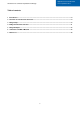
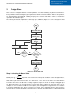
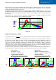
value curve (Q=1) can reach the minimum gain (K=0.8) with less switching frequency increase, but unable
to reach the maximum gain (K=1.2). Therefore, a moderate Q value of around 0.5 seems to satisfy the
voltage gain requirement in this specific case.
We conclude that adjusting the Q value can help achieving the maximum gain but increases the frequency
modulation range, thus, we should not rely on tuning the Qmax value as a design iteration in order to reach
the desired maximum voltage gain, but instead we should rely on tuning the m value as will be explained in
the next step.
Although there isn’t a direct method for selecting the optimum Q value, we should select Qmax moderately
as discussed earlier and based on the specific design in hand.
Figure 3.2
Step 2: Selecting the m Value
As mentioned above,
r
mr
L
LL
m
, m is a static parameter that we have to start the design by optimizing its
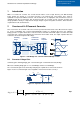
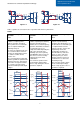
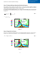
value, therefore it’s important to understand the impact of the m ratio on the converter operation. To illustrate
the effect of the m value, Figure 3.3 shows the same resonant tank gain plots but for different m values, m=
3, 6 and 12. It is obvious that lower values of m can achieve higher boost gain, in addition to the narrower
range of the frequency modulation, meaning more flexible control and regulation, which is valuable in
applications with wide input voltage range. Nevertheless, low values of m for the same quality factor Q and
resonant frequency fr means smaller magnetizing inductance Lm, hence, higher magnetizing peak-peak
current ripple, causing increased circulating energy and conduction losses.
We have to start by selecting a reasonable initial value for m (6-10), and then optimize it by few iterations to
get the maximum m value that can still achieve the maximum gain requirement for all load conditions.
Figure 3.3
Low m value:
Higher boost gain
Narrower frequency range
More flexible regulation
High m value:
Higher magnetizing inductance
Lower magnetizing circulating current
Higher efficiency
0.1 1 10
0
0.5
1
1.5
2
K .3 m Fx( )
K .5 m Fx( )
K 1 m Fx( )
1.2
0.8
Fx
0.1 1 10
0
1
2
3
K .2 m, Fx,( )
K .3 m, Fx,( )
K .5 m, Fx,( )
K .7 m, Fx,( )
K 1 m, Fx,( )
K 5 m, Fx,( )
Fx
m=12
0.1 1 10
0
1
2
3
K .2 m, Fx,( )
K .3 m, Fx,( )
K .5 m, Fx,( )
K .7 m, Fx,( )
K 1 m, Fx,( )
K 5 m, Fx,( )
Fx
m=6
x
0
.001
10
0.1 1 10
0
1
2
3
K .2 m, Fx,
(
)
K .3 m, Fx,
(
)
K .5 m, Fx,
(
)
K .7 m, Fx,
(
)
K 1 m, Fx,
(
)
K 5 m, Fx,
(
)
Fx
m=3