Calc Guide

• The search data is in descending order and the data is large
enough that the data must be searched assuming that it is sorted;
because it is faster to sort a sorted list.
Examples
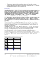
Consider the data in Table 23. Each student’s information is stored in a
single row. Write a formula to return the average grade for Fred. The
problem can be restated as Search column A in the range A1:G16 for
Fred and return the value in column F (column F is the sixth column).
The obvious solution is =VLOOKUP("Fred"; A2:G16; 6). Equally
obvious is =LOOKUP("Fred"; A2:A16; F2:F16).
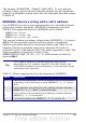
It is common for the first row in a range to contain column headers. All
of the search functions check the first row to see if there is a match
and then ignore it if it does not contain a match, in case the first row is
a header.
What if the column heading Average is known, but not the column
containing the average? Find the column containing Average rather
than hard coding the value 6. A slight modification using MATCH to
find the column yields
=VLOOKUP("Fred"; A2:G16; MATCH("Average"; A1:G1; 0)); notice
that the heading is not sorted. As an exercise, use HLOOKUP to find
Average and then MATCH to find the row containing Fred.
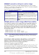
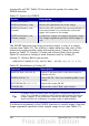
As a final example, write a formula to assign grades based on a
student’s average score. Assume that a score less than 51 is an F, less
than 61 is an E, less than 71 is a D, less than 81 is a C, less than 91 is a
B, and 91 to 100 is an A. Assume that the values in Table 20 are in
Sheet2.
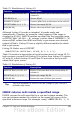
Table 20. Associate scores to a grade.
A B
1
Score Grade
2
0 F
3
51 E
4
61 D
5
71 C
6
81 B
7
91 A
382 OpenOffice.org 3.x Calc Guide