User's Manual

Chapter 4 Frequency-Weighted Error Reduction
Xmath Model Reduction Module 4-8 ni.com
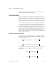
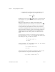
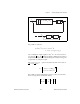
The left MFD corresponds to the setup of Figure 4-3.
Figure 4-3. C(s) Implemented to Display Left MFD Representation
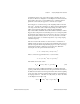
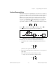
The setup of Figure 4-2 suggests approximation of:
whereas that of Figure 4-3 suggests approximation of:
In the LQG optimal case, the signal driving K
E
in Figure 4-2 is white noise
(the innovations process); this motivates the possibility of using no
frequency dependent weighting in approximating G(s) [but observe that
after approximating, the signal will no longer be white noise, so that
argument is questionable]. Simple appeal to duality motivates using no
frequency dependent weighting for H(s). These are two of the options
offered by
fracred( ).
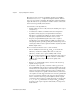
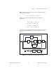
Two more
fracred( ) options depend on examining stability robustness
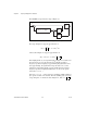
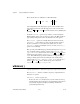
(the options are duals of one another). From the stability point of view, the
set-up of Figure 4-3 is identical to that of Figure 4-4, with .
K
r
sI A K
E
C+–()
1–
K
E
B
Ps()
+
-
Gs()
K
r
C
= sI A– BK
r
+()
1–
K
E
Hs() K
R
sI A– K
E
C+()
1–
BK
E
=
P
ˆ
PI
=