User's Manual

Chapter 3 Multiplicative Error Reduction
Xmath Model Reduction Module 3-8 ni.com
state-variable representation of G. In this case, the user is effectively asking
for G
r
= G. When the phase matrix has repeated Hankel singular values,
they must all be included or all excluded from the model, that is,
ν
nsr
= ν
nsr + 1
is not permitted; the algorithm checks for this.
The number of ν
i
equal to 1 is the number of zeros in Re[s]>0 of G(s), and
as mentioned already, these zeros remain as zeros of G
r
(s).
If
error is specified, then the error bound formula (Equation 3-2) in
conjunction with the ν
i
values from step 3 is used to define nsr for step 4.
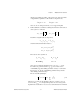
For nonsquare G with more columns than rows, the error formula is:
If the user is presented with the ν
i
, the error formula provides a basis for
intelligently choosing
nsr. However, the error bound is not guaranteed to
be tight, except when nsr = ns –1.
Securing Zero Error at DC
The error G
–1
(G – G
r
) as a function of frequency is always zero at ω = ∞.
When the algorithm is being used to approximate a high order plant by a
low order plant, it may be preferable to secure zero error at ω = 0. A method
for doing this is discussed in [GrA90]; for our purposes:
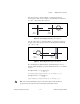
1. We need a bilinear transformation of sys = 1/z. Given G(s) we generate
H(s) through:
bilinsys=makepoly([b3,b4]/makepoly([b1,b2])
sys=subsys(sys,bilinsys)
2. Reduce with the previous algorithm:
[sr,nsr,hsv] = bst(sys)
3. Use the bilinear transformation s = 1/z again:
[sr1,nsr1] = bilinear(sr,nsr,[0,1,1,0])
The ν
i
are the same for G(s) and H(s)=G(s
–1
). The error bound formula is
the same; H is stable and H(jω)H'(–jω) of full rank for all ω including
ω = ∞ if and only if G has the same property; right half plane zeros of G are
still preserved by the algorithm. The error G
–1
(G – G
r
), though now zero at
ω = 0, is in general nonzero at ω = ∞.
GG
r
–()
*
G
*
G()
1–
GG
r
–()
∞
12⁄
2
v
i
1 v
i
–
-------------
insr1+=
ns
∑
≤