User's Manual

Chapter 2 Additive Error Reduction
Xmath Model Reduction Module 2-16 ni.com
By abuse of notation, when we say that G is reduced to a certain order, this
corresponds to the order of G
r
(s) alone; the unstable part of G
u
(s) of the
approximation is most frequently thrown away. The number of eliminated
states (retaining G
u
) refers to:
(# of states in G) – (# of states in G
r
) – (# of states in G
u
)
This number is always the multiplicity of a Hankel singular value. Thus,
when the order of G
r
is n
i –1
the number of eliminated states is n
i
– n
i –1
or
the multiplicity of σ
n
i – 1
+ 1
= σ
ni
.
For each order n
i –1
of G
r
(s), it is possible to find G
r
and G
u
so that:
(Choosing i = 1 causes G
r
to be of order zero; identify n
0
= 0.) Actually,
among all “approximations” of G(s) with stable part restricted to having
degree n
i –1
and with no restriction on the degree of the unstable part, one
can never obtain a lower bound on the approximation error than σ
n
i
; in the
scalar or SISO G(s) case, the G
r
(s) which achieves the previous bound is
unique, while in the matrix or MIMO G(s) case, the G
r
(s) which achieves
the previous bound may not be unique [Glo84]. The algorithm we use to
find G
r
(s) and G
u
(s) however allows no user choice, and delivers a single
pair of transfer function matrices.
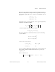
The transfer function matrix G
r
( jω) alone can be regarded as a stable
approximation of G( jω). If the D matrix in G
r
( jω) is approximately
chosen, (and the algorithm ensures that it is), then:
(2-3)
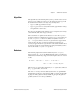
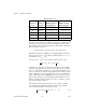
Table 2-1. Orders of G
Order of
G
r
nsr
Order of
G
u
nsu
Number of
Eliminated States
(Retaining G
u
)
Number of
Eliminated States
(Discarding G
u
)
0 ns – n
1
n
1
ns
n
1
ns – n
2
n
2
– n
1
ns – n
1
n
2
ns – n
3
n
3
– n
2
ns – n
2
⇓ ⇓ ⇓ ⇓
n
m –1
0 ns – n
m –1
ns – n
m –1
Gjω()G
r
jω()– G
u
jω()–
∞
σ
n
i
≤
Gjω()G
r
jω()–
∞
σ
n
i
σ
n
i 1+
... σ
ns
+++≤