User's Manual

Chapter 2 Additive Error Reduction
© National Instruments Corporation 2-15 Xmath Model Reduction Module
Algorithm
The algorithm does the following. The system Sys and the reduced order
system
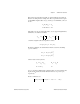
SysR are stable; the system SysU has all its poles in Re[s] > 0. If
the transfer function matrices are G(s), G
r
(s) and G
u
(s) then:
• G
r
(s) is a stable approximation of G(s).
• G
r
(s)+G
u
(s) is a more accurate, but not stable, approximation of G(s),
and optimal in a certain sense.
Of course, the algorithm works with state-space descriptions; that of G(s)
can be minimal, while that of G
r
(s) cannot be.
These statements are explained in the Behaviors section. If
onepass is
specified, reduction is calculated in one pass. If
onepass is not called or is
set to 0
{onepass=0}, reduction is calculated in (number of states of
Sys - nsr) passes. There seems to be no general rule to suggest which
setting produces the more accurate approximation G
r
. Therefore, if
accuracy of approximation for a given order is critical, both should be tried.
As noted previously, if an approximation involving an unstable system is
desired, the default
{onepass=1} is specified.
Behaviors
The following explanation deals first with the keyword {onepass}.
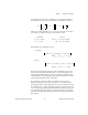
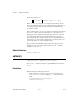
Suppose that σ
1
, σ
2
,..., σ
ns
are the Hankel Singular values of S, which has
transfer function matrix G(s). Suppose that the singular values are ordered
so that:
Thus, there are n
1
equal values, followed by n
2
– n
1
equal values, followed
by n
3
– n
2
equal values, and so forth.
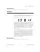
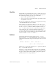
The order
nsr of G
r
(s) cannot be arbitrary when there are equal Hankel
singular values. In fact, the orders shown in Table 2-1 for the strictly stable
G
r
(all poles in Re[s]<0) and strictly unstable G
u
(all poles Re[s]>0) are
possible (and there are no other possibilities).
σ
1
σ
2
... σ
n
1
=== σ
n
1
1+
...>σ
n
1
1+
... σ
n
2
σ
n
2
1+
...>==
σ
n
m 1–
1+
σ
n
m 1–
2+
σ
n
m
=σ
ns
()0≥==>