User's Manual

Chapter 2 Additive Error Reduction
Xmath Model Reduction Module 2-12 ni.com
redschur( )
[SysR,HSV,slbig,srbig,VD,VA] = redschur(Sys,{nsr,bound})
The redschur( ) function uses a Schur method (from Safonov and
Chiang) to calculate a reduced version of a continuous or discrete system
without balancing.
Algorithm
The objective of redschur( ) is the same as that of balmoore( ) when
the latter is being used to reduce a system; this means that if the same
Sys
and
nsr are used for both algorithms, the reduced order system should have
the same transfer function matrix. However, in contrast to
balmoore( ),
redschur( ) do not initially transform Sys to an internally balanced
realization and then truncate it; nor is
SysR in balanced form. The fact that
there is no balancing offers numerical advantages, especially if
Sys is
nearly nonminimal.
Sys should be stable, and this is checked by the algorithm. In contrast to
balmoore( ), minimality of Sys (that is, controllability and
observability) is not required.
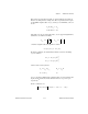
If the Hankel singular values of
Sys are ordered as ,
then those of
SysR in the continuous-time case are .
A restriction of the algorithm is that is required for both
continuous-time and discrete-time cases. Under this restriction,
SysR is
guaranteed to be stable and minimal.
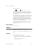
The algorithms depend on the same algorithm, apart from the calculation
of the controllability and observability grammians W
c
and W
o
of the
original system. These are obtained as follows:
The maximum order permitted is the number of nonzero eigenvalues of
W
c
W
o
that are larger than ε.
σ
1
σ
2
... σ
ns
0≥≥≥ ≥
σ
1
σ
2
... σ
nsr
0>≥≥≥
σ
nsr
σ
nsr 1+
>
(continuous)
(discrete)
W
c
A′ AW
c
+ BB′–= W
o
AA′W
o
+ C′C=
W
c
AW
c
A′– BB′= W
o
A′W
o
A– C′C=