User's Manual

Chapter 1 Introduction
© National Instruments Corporation 1-7 Xmath Model Reduction Module
• An inequality or bound is tight if it can be met in practice, for example
is tight because the inequality becomes an equality for x =1. Again,
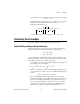
if F(jω) denotes the Fourier transform of some , the
Heisenberg inequality states,
and the bound is tight since it is attained for f(t) = exp + (–kt
2
).
Commonly Used Concepts
This section outlines some frequently used standard concepts.
Controllability and Observability Grammians
Suppose that G(s)=D + C(sI–A)
–1
B is a transfer-function matrix with
Reλ
i
(A)<0. Then there exist symmetric matrices P, Q defined by:
PA′ +AP = –BB′
QA + A′Q = –C′C
These are termed the controllability and observability grammians of the
realization defined by {A,B,C,D}. (Sometimes in the code, WC is used for
P and WO for Q.) They have a number of properties:
• P ≥ 0, with P > 0 if and only if [A,B] is controllable, Q ≥ 0 with Q >0
if and only if [A,C] is observable.
• and
• With vec P denoting the column vector formed by stacking column 1
of P on column 2 on column 3, and so on, and ⊗ denoting Kronecker
product
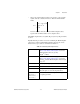
• The controllability grammian can be thought of as measuring the
difficulty of controlling a system. More specifically, if the system is in
the zero state initially, the minimum energy (as measured by the L
2
norm of u) required to bring it to the state x
0
is x
0
P
–1
x
0
; so small
eigenvalues of P correspond to systems that are difficult to control,
while zero eigenvalues correspond to uncontrollable systems.
1 xx– 0≤log+
ft() L
2
∈
ft()
2
dt
∫
t
2
∫
ft()
2
dt
12⁄
ω
2
∫
Fjω()
2
dω
12⁄
-------------------------------------------------------------------------------------------
4π≤
Pe
At
BB′e
A′t
dt
0
∞
∫
= Qe
A′t
C′Ce
At
dt
0
∞
∫
=
IAAI⊗+⊗[]vecP vec(– BB′)=