NI MATRIXx Xmath Robust Control Module TM MATRIXx Xmath Robust Control Module April 2007 370757C-01 TM
Support Worldwide Technical Support and Product Information ni.
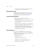
Important Information Warranty The media on which you receive National Instruments software are warranted not to fail to execute programming instructions, due to defects in materials and workmanship, for a period of 90 days from date of shipment, as evidenced by receipts or other documentation. National Instruments will, at its option, repair or replace software media that do not execute programming instructions if National Instruments receives notice of such defects during the warranty period.
Conventions The following conventions are used in this manual: [] Square brackets enclose optional items—for example, [response]. » The » symbol leads you through nested menu items and dialog box options to a final action. The sequence File»Page Setup»Options directs you to pull down the File menu, select the Page Setup item, and select Options from the last dialog box. This icon denotes a note, which alerts you to important information.
Contents Chapter 1 Introduction Using This Manual.........................................................................................................1-1 Document Organization...................................................................................1-1 Bibliographic References ................................................................................1-2 Commonly-Used Nomenclature......................................................................1-2 Related Publications ................
Contents Chapter 3 System Evaluation Singular Value Bode Plots............................................................................................. 3-1 L Infinity Norm (linfnorm)............................................................................................ 3-3 linfnorm( ) ....................................................................................................... 3-4 Singular Value Bode Plots of Subsystems ....................................................................
1 Introduction The Xmath Robust Control Module (RCM) provides a collection of analysis and synthesis tools that assist in the design of robust control systems. This chapter starts with an outline of the manual and some use notes. It continues with an overview of the Xmath Robust Control Module (RCM) functions. Using This Manual This manual provides complete documentation for all the RCM functions along with their associated theoretical background, references, and examples.
Chapter 1 Introduction techniques. The general problem setup is explained together with known limitations; the rest is left to the references. Bibliographic References Throughout this document, bibliographic references are cited with bracketed entries. For example, a reference to [DoS81] corresponds to a document published by Doyle and Stein in 1981. For a table of bibliographic references, refer to Appendix A, Bibliography.
Chapter 1 • Xmath Optimization Module • Xmath Robust Control Module • Xmath Xμ Module Introduction MATRIXx Help Robust Control Module function reference information is available in the MATRIXx Help. The MATRIXx Help includes all Robust Control functions. Each topic explains a function’s inputs, outputs, and keywords in detail. Refer to Chapter 2, MATRIXx Publications, Help, and Online Support, of the MATRIXx Getting Started Guide for complete instructions on using the Help feature.
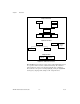
Chapter 1 Introduction Analysis Functions smargin wcbode wcgain ssv pfscale optscale osscale Synthesis Functions hinfcontr lqgltr singriccati fslqgcomp fsesti fsregu clsys Utility Functions linfnorm perfplots Figure 1-1. RCM Function Structure Many RCM functions are based on state-of-the-art algorithms implemented in cooperation with researchers at Stanford University. The robustness analysis functions are based on structured singular value calculations.
2 Robustness Analysis This chapter describes RCM tools used for analyzing the robustness of a closed-loop system. The chapter assumes that a controller has been designed for a nominal plant and that the closed-loop performance of this nominal system is acceptable. The goal of robustness analysis is to determine whether the performance will remain acceptable if the plant differs from the nominal plant. Modeling Uncertain Systems This section describes the method RCM uses to model an uncertain system.
Chapter 2 Robustness Analysis system, including how the uncertain transfer functions are connected to the system and the magnitude bound functions li (w). To do this, extract the uncertain transfer functions and collect them into a k-input, k-output transfer matrix Δ, where: Δ ( jω) = diagonal ( δ 1 ( jω),...,δ k ( jω) ) (2-2) The resulting closed-loop system can be viewed as a feedback connection of the nominal closed-loop system with transfer matrix H(jω) and the uncertain transfer matrix Δ(jω).
Chapter 2 Robustness Analysis Stability Margin (smargin) Assume that the nominal closed-loop system is stable. That belief raises a question: Does the system remain stable for all possible uncertain transfer functions that satisfy the magnitude bounds (Equation 2-1)? If so, the system is said to be robustly stable. If the magnitude bounds are small enough, the uncertainties will not destabilize the system; your system will be robustly stable.
Chapter 2 Robustness Analysis smargin( ) marg = smargin(SysH, delb {scaling, graph}) The smargin( ) function plots an approximation to the stability margin of the system as a function of frequency. For a full discussion of smargin( ) syntax, refer to the MATRIXx Help. The approximation is exact if the number of uncertain transfer functions is less than four and scaling="OPT" (optimum scaling). In other cases, the approximation is generally considered to be extremely good.
Chapter 2 Robustness Analysis reference + – error 1 + 8 – + – + x1 1 s 1 s x2 reference 2 1 + + + + K1 = 4 K2 = 8 Figure 2-3. SISO Tracking System with Three Uncertainties The H system will have the reference input as input1 and the error output as output1 (w and z, respectively, in Figure 2-2). Removing the δ values will create inputs 2 through 4 and outputs 2 through 4 (r and q, respectively, in Figure 2-2). 1.
Chapter 2 Robustness Analysis dB 10 0 –20 0.1 1 30 100 Frequency, Radian/Second Figure 2-4. Bound for Sensor Uncertainty Note A value of l3 at one radian per second of –20 dB indicates that modeling uncertainties of up to 10% (–20 dB = 0.1) are allowed. The actuator and sensor uncertainties δ1 and δ2 are bounded by –20 dB at all frequencies. You will use these values to interpolate to obtain l3. First, create the bound for δ3 in Hz. L3 = pdm([-20,-20,10,10],[0.1,1,30,100]/2/pi); 3.
Chapter 2 Robustness Analysis Figure 2-5. Stability Margin Now examine the effect on the stability margin of discretizing H(s) at 100 Hz. dt = 0.01; Hd = discretize(H,dt); margD = smargin(Hd,delb); smargin smargin smargin smargin --> --> --> --> Scaling algorithm is type: PF Margin computation 10% complete Margin computation 50% complete Margin computation 90% complete 100 Hz is a high discretization frequency for H, so the stability margin is unchanged in the discrete-time case.
Chapter 2 Robustness Analysis Worst-Case Performance Degradation (wcbode) Even if a system is robustly stable, the uncertain transfer functions still can have a great effect on performance. Consider the transfer function from the qth input, wq, to the pth output, zp. With δ1 = ... = ...δk = 0, you have the nominal system, and this transfer function is the p,q entry of Hzw. This is called the nominal transfer function.
Chapter 2 Robustness Analysis wcbode( ) [WCMAG, NOMMAG] = wcbode (SysH, delb, {input, output, graph}) The wcbode( ) function computes and plots the worst-case gain of a closed-loop transfer function. This function is useful for checking a system that already has been verified to be robustly stable using smargin( ). For example, a system can have a minimum stability margin of 4 dB, so it is robustly stable.
Chapter 2 Robustness Analysis Figure 2-6. Performance Degradation of the SISO Tracking System Advanced Topics This section describes the theoretical background on robustness analysis and performance degradation. Stability Margin This section discusses advanced aspects of computing the stability margin and the related scaling algorithms. Stability Margin and Structured Singular Values (μ) The stability margin was first defined by Safonov in [Saf82]. If you let M = H qr diagonal ( l 1 ( w ), ...
Chapter 2 Robustness Analysis for all diagonal Δ such that 1 ( Δ ii ≤ α ) } = ------------μ(M) where μ(.) is the structured singular value, introduced by Doyle in [Doy82]. Thus, the margin is the inverse of the structured singular value of Hqr diagonally scaled by the magnitude bounds. There is no numerically efficient algorithm that is guaranteed to compute μ(M), and hence the stability margin. However, it is possible to compute various good approximations to μ(M).
Chapter 2 Robustness Analysis You can compare this margin to that of the example in the Creating a Nominal System section; the following inputs produce Figure 2-7. plot ([marg,margSVD],{xlog} legend=["PF_SCALE","SVD"], ylab="Stability Margin,dB", xlab="Frequency, Hz."}) Figure 2-7. pfscale( ) versus svd Stability Margins Note The singular value approach gives results that are too conservative, suggesting that the uncertainties can destabilize the system.
Chapter 2 Robustness Analysis of generality—so, roughly speaking, it can be solved. [SD83,SD84] discusses this optimization problem. Notice that: σ max ( M ) = σ ( DMD – 1 ) for D = 1 so you have the following from Equation 2-5: σ max ( M ) ≥ μ ( M ) This inequality is thought to be nearly an equality, so that the left side is a good engineering approximation to the right side.
Chapter 2 Robustness Analysis Comparing Scaling Algorithms Using the system from the first example (Figure 2-3), you can compare the results of using the three scaling algorithms: MARG_PF=smargin(H,delb,{scaling="PF",!graph}); MARG_OS=smargin(H,delb,{scaling="OS",!graph}); MARG_OPT=smargin(H,delb,{scaling="OPT",!graph}); plot ([MARG_PF,MARG_OS,MARG_OPT],{xlog, legend=["PF","OS","OPT"],xlab="Frequency, Hz.
Chapter 2 Robustness Analysis ssv( ) [v,vD] = SSV(M, {scaling}) The ssv( ) function computes an approximation (and guaranteed upper bound) to the Scaled Singular Value of a complex square matrix M, where M can be a reducible matrix. The scaled singular value v(M) is defined by: v( M) = –1 σ ( DMD ) inf D∈C n×n , det ( D ) ≠ 0, dia gonal Scaling can be accomplished with one of three algorithms: • Perron-Frobenius—If {scaling="PF"} Safonov’s Perron-Frobenius method [Saf82] is used.
Chapter 2 Robustness Analysis VOPT=ssv(M,{scaling="OPT"}) VOPT (a scalar) = 2.43952 VSVD = max(svd(M)) VSVD (a scalar) = 2.65886 osscale( ) [v, vD] = osscale(M) The osscale( ) function scales a matrix using the Osborne Algorithm. A diagonal scaling DOS is found that minimizes the Frobenius norm of –1 D OS MD OS , which is the square root of the sum of the squares of its singular values. If M is reducible, osscale( ) may encounter a divide by zero.
Chapter 2 Robustness Analysis optscale( ) [v, vOPTD] = optscale (M, {tol}) The optscale( ) function optimally scales a matrix. An iterative optimization (ellipsoid) algorithm which calculates upper and lower bounds on the left side of Equation 2-5 is used. If these bounds are within a relative accuracy you have specified (tol), optscale( ) stops.
Chapter 2 Robustness Analysis δ1 δ4 δ2 Figure 2-10. Reduction to Separate Systems In terms of the approximations to the margin discussed above, this reducibility will manifest itself as a problem such as divide-by-zero or nontermination. It really means that the minimum of the optimization problem is not achieved by any finite scaling. A matrix M can be split into its reducible components using the following technique (refer to[BeP79]): 1.
Chapter 2 Robustness Analysis Using this relation and any of the previously discussed approximations for μ(.), you can compute an approximation to wcgain( ). Because the approximations to μ(.) are upper bounds, the resulting approximations to wcgain( ) also are upper bounds. For speed purposes, wcgain( ) uses Perron-Frobenius scaling to calculate the approximation of μ.
3 System Evaluation This chapter describes system analysis functions that create singular value Bode plots, performance plots, and calculate the L∞ norm of a linear system. Singular Value Bode Plots The singular value Bode plot is a MIMO generalization of the bode( ) magnitude plot.
Chapter 3 System Evaluation Refer to [BoB91] in Appendix A, Bibliography. Example 3-1 Creating a Singular Value Plot 1. Let a system H be a 2-input/2-output system: tf=makepoly([1,2],"s")/... polynomial([0,-2.334,-12],"s") tf (a transfer function) = s + 2 -------------------(s + 2.334)(s + 12)s System is continuous H = [tf, 2*tf; tf*tf, tf+3]; [outputs,inputs]=size(H) outputs (a scalar) = inputs (a scalar) = 2. 2 2 Now plot the singular values of the system between 0.
Chapter 3 System Evaluation Figure 3-1. Singular Value Plot L Infinity Norm (linfnorm) The L∞ norm of a stable transfer matrix H is defined as: H ∞ = sup σ ( H ( jω) ) ω∈ℜ where σ is the maximum singular value and H(jω) is the transfer matrix under consideration. The L∞ norm of a stable transfer matrix is the maximum of the maximum singular values over frequency. For example, the highest point of its singular values plot. Observe that the L∞ norm can be calculated even if H is not stable.
Chapter 3 System Evaluation factor by which the RMS value of a signal flowing through H can be increased. By comparison, the H2 norm is defined as: ∞ H 1 -----2π = 2 k ∫ ∑ σ ( H ( jω) ) dw 2 i –∞ i = 1 This norm can be interpreted as the RMS value of the output when the input is unit intensity white noise. It can be computed in Xmath using the rms( ) function.
Chapter 3 • System Evaluation If A has an imaginary eigenvalue at jω0, linfnorm( ) returns: vOMEGA = ω 0 SIGMA = Infinity where ω0 is one of the imaginary eigenvalues of A. • Even if H is unstable, linfnorm( ) returns its maximum singular value on the jω axis. For discrete-time systems linfnorm( ) converts a discrete-time L∞ norm computation problem to a continuous-time problem using a Cayley transformation.
Chapter 3 System Evaluation Figure 3-2. Singular Values of H(jω) as a Function of ω Note sv is returned in dBs. Check that sigma is within 0.01 (the default value of tol) of 10**(max(sv,{channels})/20). [sigma,10^(max(sv,{channels})/20)] ans (a row vector) = 5.07322 4.98731 The linfnorm( ) function also can be used on discrete-time systems. Consider a state-space system with a sample rate of 10 Hz: SysD=system([0.5,0.5;0.8,0.5],[0.8,0.5]', [0,1],0,{dt=0.
Chapter 3 System Evaluation Singular Value Bode Plots of Subsystems To evaluate the performance achieved by a given controller rapidly, it is useful to check four basic maximum singular value plots—for example, the transfer matrices from process and sensor noises to the error and actuator signals. perfplots( ) SV = perfplots ( Sys, nd, ne, { keywords } ) The perfplots( ) function plots the maximum singular value of the four transfer matrices of the system in the following figure.
Chapter 3 System Evaluation The four transfer matrices are labeled e/d, e/n, u/d, and u/n in the final plot. The plots in the top row, consisting of e/d and e/n, show the regulation or tracking achieved by the controller. If both these quantities are small, then the disturbance d and the sensor noise n will not make the error signal e large. The bottom row of plots, consisting of u/d and u/n, show the actuator effort used by the controller.
Chapter 3 System Evaluation The system matrix can be calculated using the afeedback( ) function for different values of K. Consider two cases: K = 1 and K = 5. P = 1/makepoly([1,0],"s") P (a transfer function) = 1 -s System is continuous K1= 1/makepoly(1,"s") K1 (a transfer function) = 1 1 System is continuous K5= 5/makepoly(1,"s"); Sys1 = afeedback(P,K1); Sys5 = afeedback(P,K5); The effect of the value of K on closed-loop performance can be investigated using perfplots( ).
Chapter 3 System Evaluation Figure 3-5. Perfplots( ) for K = 1 and K = 5 clsys( ) SysCL = clsys( Sys, SysC ) The clsys( ) function computes the state-space realization SysCL, of the closed-loop system from w to z as shown in Figure 3-6. w u Sys z y SysC Figure 3-6. Closed Loop System from w to z MATRIXx Xmath Robust Control Module 3-10 ni.
Chapter 3 System Evaluation Where SysC=system(Ac,Bc,Cc,Dc), Sys=system(A,B,C,D), and nz is the dimension of z and nw is the dimension of w : nw B is Bw Bu nw nz C is C z ,C y D is D zw D zu nz D yw D yu Given the above, SysCL is calculated as shown in Figure 3-7.
Chapter 3 System Evaluation + + 1 +1 s Figure 3-8. Ill-Posed Feedback System Example 3-4 Example of Closed-Loop System a = 1; b = [1,0,1]; c = b'; d = [0,0,0;0,0,1;0,1,0]; Sys = SYSTEM(a,b,c,d); SysC = SYSTEM(-40,2.7,-40,0); SysCL = clsys(Sys,SysC) SysCL (a state space system) = A 1 -40 2.7 -40 B 1 0 0 2.7 C 1 0 0 -40 D 0 0 0 0 X0 0 0 System is continuous MATRIXx Xmath Robust Control Module 3-12 ni.
4 Controller Synthesis This chapter discusses synthesis tools in two categories, H∞ and H2. This chapter does not explain all of the theory of H∞, LQG/LTR, and frequency shaped LQG design techniques. The general problem setup is explained together with known limitations. H-Infinity Control Synthesis Problem Definition The H∞ control synthesis function hinfcontr( ) finds a stabilizing multivariable controller K for the plant P, as shown in Figure 4-1.
Chapter 4 Controller Synthesis The function hinfcontr( ) can be used to find an optimal H∞ controller K that is arbitrarily close to solving: min H ew ∞ ≤ γ = γ opt (4-2) K The hinfcontr( ) function description in the hinfcontr( ) section describes how the optimum can be found manually by decreasing γ until an error condition occurs, or conversely by increasing γ until the error condition is fixed.
Chapter 4 Controller Synthesis Equivalently, as a transfer matrix: P( s) = D 11 D 12 D 21 D 22 + C1 C2 –1 ( sI – A ) [ B 1 B 2 ] To enter the extended system, you must know the sizes of e and w shown in Figure 4-1. The extended plant P can be constructed using the Xmath interconnection functions, as shown in Example 4-1. Building the Plant Model The general form of the plant P is shown in Figure 4-2. Plant P v w z Win Wout e G u y Figure 4-2.
Chapter 4 Controller Synthesis The transfer matrix G can be viewed as a model of the underlying system dynamics with v and u as generalized forces that produce effects in the performance signals z and measured signals y. The weight Win is used to model the exogenous input v by v = Winw. Similarly, the critical performance variables in the vector z are weighted to form the normal critical variables e = Wout z.
Chapter 4 Controller Synthesis here the weighting matrices are transfer matrices, whereas in the LQG setup they are constants.
Chapter 4 Controller Synthesis Selecting these weights has much the same effect here. Specifically, let Hzv be the closed-loop transfer matrix (with u = Kγ) from inputs: v = d n to outputs: z = y reg u Thus, H zv = H y reg d H yreg n H ud H un Suppose that the controller u = Ky approximates Equation 4-2. Thus, Wout H zv W in ∞ ≈ γ opt In many cases, this means that the maximum singular value of the frequency response matrix (Wout HzvWin)( jω) is constant over all frequencies.
Chapter 4 Controller Synthesis where M ( ω ) = max { m 11 ( u ),m 12 ( u )m 21 ( u )m 22 ( u ) } and m 11 = σ max [ W reg H yreg d W dist ] m 12 = σ max [ W reg H yreg n W noise ] m 21 = σ max [ W act H ud W dist ] m 22 = σ max [ W act H un W noise ] The weights also can be viewed as “design knobs” (for example, [ONR84]).
Chapter 4 Controller Synthesis • For all ω ≥ 0, rank A – jωI B 2 rank A – jωI B 1 C1 D 12 = NS + NU • C2 D 21 = NS + NY Condition 1 is a standard condition to ensure the existence of a stabilizing controller. Condition 2 ensures that the control signal u is contained in the normalized error vector e (refer to Figure 4-3). Conversely, condition 3 ensures that some exogenous input (disturbance or noise) affects the measured signals (refer to Figure 4-3).
Chapter 4 Controller Synthesis If no error message occurs, then H ew ∞ ≤ γ is guaranteed. However, this does not preclude the possibility that either H ew ∞ « γ or that γ opt « H ew ∞ . For the former case, there are two checks: • Use the linfnorm( ) function to compute H ew • Compute the graph σ max [ H ew ( jω ) ] versus ω. If H ew again. ∞ ∞ . « γ by about 6 dB or more, then you can decrease gamma and try When gamma is very large, the specification (Equation 4-1) is easily met.
Chapter 4 Controller Synthesis Suppose the input/output weights are as follows: 1 ----------- 0 W in = s + 1 0 0.1 2. W out = 1 0 0 0.1 Create the four weights: Wdist = 1/makepoly([1,1],"s") Wdist (a transfer function) = 1 ----s + 1 Wnoise = 0.1; Wreg=1/makepoly(1,"s"); Wact = 0.1; 3.
Chapter 4 4. Controller Synthesis For this example, you will start with gamma=1 as the initial guess and enter: [K,Hew] = hinfcontr(P,1,2,2); No error messages are reported. This means that a stabilizing controller has been found such that Equation 4-1 holds. That is, H ew ∞ ≤ 1 . The actual H∞ norm is found from: normHew=linfnorm(Hew) normHew (a scalar) = 0.211984 The result is that on this first iteration: gamma = 1 Æ normHew = 0.
Chapter 4 Controller Synthesis Figure 4-5. Perfplots for Hew It also is useful to perform perfplots( ) on the unweighted closed-loop system, Hzv, which in this case is the closed-loop transfer matrix from (d,n) into (x,u). The following function calls produce Figure 4-6: Hzv=clsys(G,K); Hzv=perfplots(Hzv,1,1,{vF=domain(svHew)}); MATRIXx Xmath Robust Control Module 4-12 ni.
Chapter 4 Controller Synthesis Figure 4-6. Perfplots for Hzv singriccati( ) [P, solstat] = singriccati(A,Q,R {method}) The singriccati( ) function solves the Indefinite Algebraic Riccati Equation (ARE): A ′ P + PA – PRP + Q = 0 The ARE is solved by decomposing the Hamiltonian: A –R –Q –A ′ The required decomposition of the Hamiltonian can be achieved using method="eig" or method="schur". The Schur decomposition is slower, but might handle some ill-conditioned problems.
Chapter 4 Controller Synthesis Linear-Quadratic-Gaussian Control Synthesis The H2 Linear-Quadratic-Gaussian (LQG) control design methods are based on minimizing a quadratic function of state variables and control inputs. Conventionally, the problem is specified in the time domain. By converting the LQG performance index into the frequency domain, it becomes obvious that the conventional LQG places equal penalty on states and control inputs at all frequencies.
Chapter 4 Controller Synthesis This expression can be converted into the following form [Gu80]: x A 21 A 22 x′ B1 + Ac Bc x +D v x′ { 0 C 12 ⎧ ⎪ ⎨ ⎪ ⎩ u = v B2 ⎧ ⎨ ⎩ A 11 A 12 ⎧ ⎪ ⎨ ⎪ ⎩ x· = x· ′ Cc Dc If R(jω) is not a function of frequency, then C12 = 0 and D = I. Note The system has a new input v and the old input u is now the output of the system. This structure is only used for computational convenience.
Chapter 4 Controller Synthesis fsesti( ) [SysF, vEV] = fsesti(SysA, ns, QWWA, QVVA, {QWVA}) The fsesti( ) function computes a frequency-shaped state estimator.
Chapter 4 Controller Synthesis fslqgcomp( ) [SysCC, vEV] = fslqgcomp(SysF, SysC) The fslqgcomp( ) function combines filter and control law to compute a controller from a control law and an estimator. For more information on the fslqgcomp( ) syntax, refer to the Xmath Help. Frequency-Shaped Control Design Commands This extended example uses the previously discussed functions to demonstrate frequency-shaped control design techniques.
Chapter 4 Controller Synthesis -0.500025 + 0.866011 j -0.500025 - 0.866011 j 5. Try the LQG compensator with the full-order system: [Syscl_fo]=feedback(Sys,Sysc); poles(Syscl_fo) ans (a column vector) = -0.401519 + 0.864869 -0.401519 - 0.864869 -0.638796 + 0.855861 -0.638796 - 0.855861 0.0152647 + 4.90994 0.0152647 - 4.90994 6. j j j j j j Find a stabilizing reduced order controller using frequency shaping.
Chapter 4 0 0 0 0 0 0 Controller Synthesis 1 0 B 0 0 0 1 C 0 D 0 0 1 0 X0 0 0 0 0 System is continuous 7. Frequency-weight the control signal. Transfer the weight on U from RUU to the third diagonal entry in RXXA. Note In Equation 4-3, u is the third state of the augmented system. RUU weighs the new frequency-shaped control signal v. Design a frequency-shaped regulator: rxxa=diagonal([0,1,1,0]);ruua=1; [Sysfs_sr,,fs_evr]=fsregu(Sysa,2,rxxa,ruua) Sysfs_sr (a state space system) = A 0 1 -1.
Chapter 4 Controller Synthesis System is continuous fs_evr (a column vector) = -0.645263 + 0.587929 j -0.645263 - 0.587929 j -0.347592 + 1.09155 j -0.347592 - 1.09155 j 8. Calculate the frequency-shaped estimator: Sysaf=system(ar,br,cr,0);qwwa=qxx;qvva=quu; [Sysfs_se,fs_eve]=fsesti(Sysaf,2,qwwa,qvva) Sysfs_se (a state space system) = A 0 1 -1 -1.00005 B 5.52357e-17 0.99005 C 1 0 0 1 D 0 0 0 0 0 1 X0 0 0 System is continuous fs_eve (a column vector) = -0.500025 + 0.866011 j -0.500025 - 0.
Chapter 4 9. Controller Synthesis Design the LQG compensator. [Sysfs_sc,fs_evc]=fslqgcomp(Sysfs_se,Sysfs_sr) Sysfs_sc (a state space system) = A 0 -1 0 0.951712 1 -1.00005 0 -0.228069 0 1 0 -1.95171 0 0 1 -1.97571 B 5.52357e-17 0.99005 0 0 C 0 0 1 0 D 0 X0 0 0 0 0 System is continuous fs_evc (a column vector) = -0.373302 -1.17564 -0.713411 + 1.33028 j -0.713411 - 1.
Chapter 4 Controller Synthesis 10. Compute the closed-loop system for the reduced order plant and the frequency-shaped compensator: [Sysfs_scl]=feedback(Sysr,Sysfs_sc); poles(Sysfs_scl) ans (a column -0.645263 + -0.645263 -0.500025 + -0.500025 -0.347592 + -0.347592 - vector) = 0.587929 j 0.587929 j 0.866011 j 0.866011 j 1.09155 j 1.09155 j 11. Compute the closed-loop system for the full-order plant and the frequency-shaped compensator.
Chapter 4 Controller Synthesis Plant G(s) y u x = Ax + Bu y = Cx x Estimator KR x = Ax + Bu + KEε ε = y – Cx x K(s) Figure 4-8. LQG Feedback System for Loop Transfer Recovery lqgltr( ) [SysC,EV,Kr] = lqgltr(Sys,Wx,Wy,K,rho,{keywords}) The lqgltr( ) function designs an estimator or regulator which recovers loop transfer robustness through the design parameter ρ (rho). For a discussion of the syntax and a full listing of keywords, refer to the Xmath Help.
Chapter 4 Controller Synthesis Then ρ is increased so that pointwise in s: –1 K ( s )G ( s ) → K R ( sI – A ) B Regulator recovery is only guaranteed if G(s) is minimum-phase and there are at least as many control signals u as measurements y.
A Bibliography [BBK88] S. Boyd, V. Balakrishnan, and P. Kabamba. “A bisection method for computing the L∞ norm of a transfer matrix and related problems.” Mathematical Control Signals, Systems Vol. 2, No. 3, pp 207–219, 1989. [BeP79] A. Berman and R.J. Plemmons. “Nonnegative Matrices in the Mathematical Sciences.” Computer Science and Applied Mathematics Series, Academic Press, 1979. [BoB90] S. Boyd and V. Balakrishnan.
Appendix A Bibliography [FaT88] M.K. Fan and A.L. Tits. “m-form Numerical Range and the Computation of the Structured Singular Value.” IEEE Transactions on Automatic Control, Vol. 33, pp 284–289, March 1988. [FaT86] M.K. Fan and A.L. Tits. “Characterization and Efficient Computation of the Structured Singular Value.” IEEE Transactions on Automatic Control, Vol. AC-31, pp 734–743, August 1986. [Fr87] B. Francis. A Course in L∞ Control Theory. Springer-Verlag, Berlin-New York, 1987. [FPGM87] D.S.
Appendix A Bibliography [SA88] G. Stein and M. Athans. “The LQG/LTR Procedure for Multivariable Control Design.” IEEE Transactions on Automatic Control, Vol. AC-32, No. 2, pp 105–114, February 1987. [Za81] G. Zames. “Feedback and optimal sensitivity: model reference transformations, multiplicative semi-norms, and approximate inverses.” IEEE Transactions on Automatic Control, Vol. AC-26, pp 301–320, 1981. [KS72] H. Kwakernaak and R. Sivan. Linear Optimal Control Systems. Wiley, 1972.
Technical Support and Professional Services B Visit the following sections of the National Instruments Web site at ni.com for technical support and professional services: • Support—Online technical support resources at ni.
Index A clsys( ), 3-10 conventions used in the manual, iv problem definition, 4-1 restrictions on extended plant, 4-7 weight selection, 4-5 H2 control synthesis, 4-14 H2 norm, 3-4 help, technical support, B-1 hinfcontr( ), 4-2, 4-8 D I diagnostic tools (NI resources), B-1 documentation conventions used in the manual, iv NI resources, B-1 drivers (NI resources), B-1 instrument drivers (NI resources), B-1 Algebraic Riccati Equation (ARE), 4-13 C K KnowledgeBase, B-1 L E L∞ norm, 3-3 linfnorm( ), 3
Index software (NI resources), B-1 ssv( ), 2-15 stability margin, 2-3, 2-10 structured nonparametric uncertainty, 2-1 structured singular value, 2-11 support, technical, B-1 system feedback connection, 2-2 nominal closed-loop, 2-1 creating, 2-4 magnitude bounds, 2-2 stability margin, 2-3 nominal transfer function, 2-8 norm H2, 3-4 L∞, 3-3 O optscale( ), 2-17 osscale( ), 2-16 P perfplots( ), 3-7 pfscale( ), 2-16 programming examples (NI resources), B-1 T technical support, B-1 training and certification