User`s manual

Lake Shore MTD Series Cryotest System User’s Manual
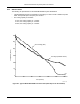
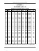
J-2 Standard Curve 10
POLYNOMIAL REPRESENTATION
Curve 10 can be expressed by a polynomial equation based on the Chebychev polynomials. Four separate ranges are
required to accurately describe the curve. Table 1 lists the parameters for these ranges. The polynomials represent
Curve 10 on the preceding page with RMS deviations of 10 mK. The Chebychev equation is:
Tx at x
ii
i
n
()
=
()
=
∑
0
(1)
where T(x)
= temperature in kelvin, t
i
(x) = a Chebychev polynomial, and a
i
= the Chebychev coefficient. The parameter x is
a normalized variable given by:
x
VVL VUV
VU VL
=
−
()
−−
()
−
()
(2)
where V = voltage and VL and VU = lower and upper limit of the voltage over the fit range. The Chebychev polynomials
can be generated from the recursion relation:
tx xtxtx
tx tx x
iii+−
()
=
()
−
()
()
=
()
=
11
01
2
1,
(3)
Alternately, these polynomials are given by:
tx i x
i
()
=×
()




cos arccos
(4)
The use of Chebychev polynomials is no more complicated than the use of the regular power series and they offer
significant advantages in the actual fitting process. The first step is to transform the measured voltage into the normalized
variable using Equation 2. Equation 1 is then used in combination with equations 3 and 4 to calculate the temperature.
Programs 1 and 2 provide sample BASIC subroutines which will take the voltage and return the temperature T calculated
from Chebychev fits. The subroutines assume the values VL and VU have been input along with the degree of the fit. The
Chebychev coefficients are also assumed to be in any array A(0), A(1),..., A(i
degree
).
An interesting property of the Chebychev fits is evident in the form of the Chebychev polynomial given in Equation 4. No
term in Equation 1 will be greater than the absolute value of the coefficient. This property makes it easy to determine the
contribution of each term to the temperature calculation and where to truncate the series if full accuracy is not required.

FUNCTION Chebychev (Z as double)as double
REM Evaluation of Chebychev series
X=((Z-ZL)-(ZU-Z))/(ZU-ZL)
Tc(0)=1
Tc(1)=X
T=A(0)+A(1)*X
FOR I=2 to Ubound(A())
Tc(I)=2*X*Tc(I-1)-Tc(I-2)
T=T+A(I)*Tc(I)
NEXT I
Chebychev=T
END FUNCTION
FUNCTION Chebychev (Z as double)as double
REM Evaluation of Chebychev series
X=((Z-ZL)-(ZU-Z))/(ZU-ZL)
T=0
FOR I=0 to Ubound(A())
T=T+A(I)*COS(I*ARCCOS(X))
NEXT I
Chebychev=T
END FUNCTION
NOTE:
arccos arctanX
X
X
()
=−
−






π
2
1
2
Program 1. BASIC subroutine for evaluating the temperature
T from the Chebychev series using Equations (1) and (3). An
array T
c
(i
degree
) should be dimensioned. See text for details.
Program 2. BASIC subroutine for evaluating the temperature T
from the Chebychev series using Equations (1) and (4). Double
precision calculations are recommended.

Table 1. Chebychev Fit Coefficients
2.0 K to 12.0 K
12.0 K to 24.5 K 24.5 K to 100.0 K 100 K to 475 K
VL = 1.32412
VU = 1.69812
A(0) = 7.556358
A(1) = –5.917261
A(2) = 0.237238
A(3) = –0.334636
A(4) = –0.058642
A(5) = –0.019929
A(6) = –0.020715
A(7) = –0.014814
A(8) = –0.008789
A(9) = –0.008554
VL = 1.11732
VU = 1.42013
A(0) = 17.304227
A(1) = –7.894688
A(2) = 0.453442
A(3) = 0.002243
A(4) = 0.158036
A(5) = –0.193093
A(6) = 0.155717
A(7) = –0.085185
A(8) = 0.078550
A(9) = –0.018312
A(10) = 0.039255
VL = 0.923142
VU = 1.13935
A(0) = 71.818025
A(1) = –53.799888
A(2) = 1.669931
A(3) = 2.314228
A(4) = 1.566635
A(5) = 0.723026
A(6) = –0.149503
A(7) = 0.046876
A(8) = –0.388555
A(9) = 0.056889
A(10) = 0.116823
A(11) = 0.058580
VL = 0.079767
VU = 0.999614
A(0) = 287.756797
A(1) = –194.144823
A(2) = –3.837903
A(3) = –1.318325
A(4) = –0.109120
A(5) = –0.393265
A(6) = 0.146911
A(7) = –0.111192
A(8) = 0.028877
A(9) = –0.029286
A(10) = 0.015619