Specifications

6.1 Amplitude dependent signal shaping 59
s~ A
s~ B
sig~ 1
phasor~ 640
/~
+~ 1
pd grapha
B
pd grapha
A
fig 6.5: Signal reciprocal
For a signal a in the range 0.0 to x the re-
ciprocal is defined as 1/a. When a is very
large then 1/a is close to ze ro, and when a
is close to zero then 1/a is very large. Usu-
ally, since we are dealing with normalised
signals, the largest input is a = 1.0, so be-
cause 1/1.0 = 1.0 the reciproc al is also 1.0.
The graph of 1/a for a between 0.0 and 1.0 is a curve, so a typical use of the
reciprocal is shown in Fig. 6.5. A curve is produced according to 1/(1 + a).
Since the maximum amplitude of the divisor is 2.0 the minimum of the output
signal is 0.5.
Limits
Sometimes we want to constrain a signal within a certain range. The
min~
unit outputs the minimum o f its two inlets or arguments. Thus
min~ 1
is the
minimum of one and w hatever signal is on the left inlet, in other words it clamps
the signal to a maximum value of one if it excee ds it. Conversely
max~ 0
returns
the maximum of zero and its signal, which means that signals g oing below zero
are clamped there forming a lower bound. You can see the effect of this on a
cosine signal in Fig. 6.6.
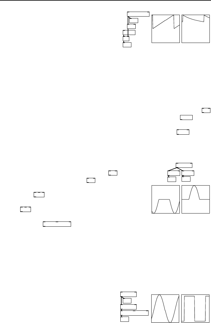
osc~ 640
max~ 0min~ 0
s~ A
s~ B
pd grapha
B
pd grapha
A
fig 6.6: Min and max of a
signal
Think about this carefully, the terminology seems to
be reversed but it is correct. You use
max~
to create
a minimum possible value and
min~
to cr eate a maxi-
mum possible value. There is a slightly les s confusing
alternative
clip~
for situations where you don’t want
to adjust the limit using another sig nal. The left in-
let of
clip~
is a signal and the remaining two inlets
or a rguments are the values of upper and lower limits,
so for example
clip~ -0.5 0.5
will limit any signal into a
range of one centered about zero.
Wave shaping
Using these principles we can start with one waveform a nd apply operations
to create others like square, triangle, pulse or any other shape. The choice of
starting waveform is usually a phasor, since anything can be derived from it.
Sometimes it’s b e st to minimise the number of operations so a cosine wave is
the best starting point.
*~ 1e+09
osc~ 640
clip~ -0.9 0.9
s~ A
s~ B
pd grapha
B
pd grapha
A
fig 6.7: Square wave
One method of making a square wave is
shown in Fig. 6.7. An ordinary cosine o s-
cillator is multiplied by a large number
and then clipp ed. If you picture a graph
of a greatly magnified cosine waveform its
slope will have become e xtremely steep,
crossing through the area between −1.0
and 1.0 almost vertically. Once clipped to a normalised range what remains is