743 Rancimat Manual 8.743.
Metrohm AG CH-9100 Herisau Switzerland Phone +41 71 353 85 85 Fax +41 71 353 89 01 info@metrohm.com www.metrohm.com 743 Rancimat Manual 8.743.8003EN 03.
Teachware Metrohm AG CH-9100 Herisau teachware@metrohm.com This documentation is protected by copyright. All rights reserved. Although all the information given in this documentation has been checked with great care, errors cannot be entirely excluded. Should you notice any mistakes please send us your comments using the address given above. Documentation in additional languages can be found on http://products.metrohm.com under Literature/Technical documentation.
■■■■■■■■■■■■■■■■■■■■■■ Table of contents Table of contents 1 Introduction 1 1.1 Instrument description ......................................................... 1 1.2 Rancimat method ................................................................. 2 1.3 About the documentation ................................................... 3 1.3.1 Symbols and conventions ........................................................ 3 1.4 Safety instructions ..........................................................
■■■■■■■■■■■■■■■■■■■■■■ Table of contents 4.1.7 4.1.8 Mouse functions .................................................................... 31 Help ...................................................................................... 32 4.2 Instrument and Program Settings ..................................... 33 4.2.1 Establishing the instrument communication ........................... 33 4.2.2 Managing access rights ......................................................... 34 4.2.3 Timer ..............
■■■■■■■■■■■■■■■■■■■■■■ Table of contents 5 Handling and maintenance 160 5.1 General information ......................................................... 160 5.1.1 Care .................................................................................... 160 5.1.2 Maintenance by Metrohm Service ........................................ 160 5.2 Replacing the dust filter .................................................. 161 5.3 Regenerating or replacing the molecular sieve ............. 161 5.
■■■■■■■■■■■■■■■■■■■■■■ Table of figures Table of figures Figure 1 Figure 2 Figure 3 Figure 4 Figure 5 Figure 6 Figure 7 VI ■■■■■■■■ Measuring arrangement (schematic representation) ........................... 3 Front 743 Rancimat ........................................................................... 7 Rear 743 Rancimat ............................................................................ 8 Mounting accessories for the air supply (rear of the instrument) ......
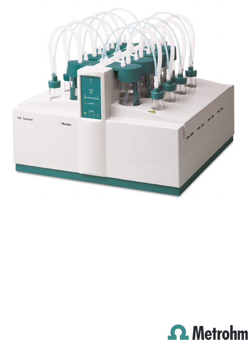
■■■■■■■■■■■■■■■■■■■■■■ 1 Introduction 1 Introduction 1.1 Instrument description The 743 Rancimat is a PC-controlled measuring device for determining the oxidation stability of samples containing oil and fat. It is equipped with two heating blocks each with 4 measuring positions (channels). Every block can be heated individually, i.e. 4 samples can each be measured at 2 different temperatures or 8 samples at the same temperature.
■■■■■■■■■■■■■■■■■■■■■■ 1.2 Rancimat method offers a GLP test set to carry out these tests (see Optional accessories, page 185). 1.2 Rancimat method The decay of vegetable and animal fats, which can be perceived in the initial stage through a deterioration of odor and taste (rancidity), is to a great extent the result of chemical alterations caused by the effect of atmospheric oxygen. These oxidation processes progressing slowly at ambient temperatures are referred to as autoxidation.
■■■■■■■■■■■■■■■■■■■■■■ 1 Introduction Measuring vessel Conductivity measuring cell Measuring solution Reaction vessel Sample Heating block Figure 1 1.3 Measuring arrangement (schematic representation) About the documentation Caution Please read through this documentation carefully before putting the instrument into operation. The documentation contains information and warnings which have to be followed by the user in order to ensure safe operation of the instrument. 1.3.
■■■■■■■■■■■■■■■■■■■■■■ 1.4 Safety instructions [Next] Button or key Warning This symbol draws attention to a possible life hazard or risk of injury. Warning This symbol draws attention to a possible hazard due to electrical current. Warning This symbol draws attention to a possible hazard due to heat or hot instrument parts. Warning This symbol draws attention to a possible biological hazard. Caution This symbol draws attention to a possible damage of instruments or instrument parts.
■■■■■■■■■■■■■■■■■■■■■■ 1 Introduction Flammable substances Warning The oven of the 743 Rancimat can be heated to 220 °C. Flammable substances may ignite at these temperatures. Adjust the maximum heating temperature of the oven to the sample being examined. Defective glass vessels Warning Caution with defective glass vessels. An overflow of flammable samples into the heating block can be dangerous. Check the glass vessels before each use. 1.4.
■■■■■■■■■■■■■■■■■■■■■■ 1.4 Safety instructions Mains voltage Warning An incorrect mains voltage can damage the instrument. Only operate this instrument with a mains voltage specified for it (see rear panel of the instrument). Protection against electrostatic charges Warning Electronic components are sensitive to electrostatic charges and can be destroyed by discharges.
■■■■■■■■■■■■■■■■■■■■■■ 2 Overview of the instrument 2 Overview of the instrument 6 1 7 2 8 3 9 4 10 5 11 743 Rancimat Figure 2 743 Rancimat Front 743 Rancimat ■■■■■■■■ 7
■■■■■■■■■■■■■■■■■■■■■■ 1 Pilot lamp Lights up when the instrument is switched on. 2 Gas flow display Flashes when the gas flow is switched on. Lights up when the gas flow has been reached. 3 Temperature display Flashes when the heating is switched on. Lights up when the temperature has been reached. 4 Error display (red) Lights up or flashes when a fault has occurred in the instrument (see Troubleshooting Chapter). 5 Instrument number display Indicates the number of the instrument.
■■■■■■■■■■■■■■■■■■■■■■ 2 Overview of the instrument 1 Collection tube holder For fastening the optional exhaust collection tube (6.2757.000). 2 Electrode connector For connecting the conductivity measuring cell integrated in the measuring vessel cover (2-7). 3 Air supply connection For connecting the FEP tubing 250 mm (2-6). 4 Mains switch For turning the instrument on and off. 5 Mains connection socket For important information on the mains connection, see Chapter 3.3.
■■■■■■■■■■■■■■■■■■■■■■ 3.1 Setting up the instrument 3 Installation 3.1 Setting up the instrument 3.1.1 Packaging The instrument is supplied in highly protective special packaging together with the separately packed accessories. Keep this packaging, as only this ensures safe transportation of the instrument. 3.1.2 Checks Immediately after receipt, check whether the shipment has arrived complete and without damage by comparing it with the delivery note. 3.1.
■■■■■■■■■■■■■■■■■■■■■■ 3 Installation Molecular sieve flask 8 Filter 1 From flask To flask 9 2 Air out 10 3 11 Air/N2 in 4 Figure 4 5 6 12 7 Mounting accessories for the air supply (rear of the instrument) 1 Drying flask cover (6.1602.145) Cover for the drying flask. 2 Drying flask (6.1608.050) 3 Flask holder For fastening the drying flask. 4 Filter tube (6.1821.040) 5 FEP tubing 250 mm (6.1805.080) For supplying the air from the internal pump to the drying flask.
■■■■■■■■■■■■■■■■■■■■■■ 3.2 Mounting accessories Note The dust filter serves for filtering the air sucked through the air pump and must be replaced at periodic intervals (see Chapter 5.2, page 161). 2 Mount drying flask Caution Do not fill the hot molecular sieve directly into the drying flask after regeneration, as otherwise the plastic filter on the filter tube will melt. Wait until the molecular sieve has cooled down before filling. ■ ■ ■ ■ ■ ■ ■ Fill the molecular sieve into the drying flask (4-2).
■■■■■■■■■■■■■■■■■■■■■■ 3 Installation ■ 3.2.2 Screw the other end of the FEP tubing onto the Air/N2 in connection (4-12). Mounting accessories for the external air supply If the laboratory air is heavily contaminated, an external gas supply with synthetic air can be provided. For this, the corresponding accessories must be mounted on the rear of the Rancimat.
■■■■■■■■■■■■■■■■■■■■■■ 3.
■■■■■■■■■■■■■■■■■■■■■■ 3 Installation 1 FEP tubing 250 mm (6.1805.080) For supplying air into the reaction vessel. 2 Silicone tubing (6.1816.010) For connecting the reaction vessel to the measuring vessel. 3 Thread adapter M8 / M6 (6.1808.090) 4 Tubing connector For connecting the silicone tubing. 5 Air tube (6.2418.100) 6 O-ring (6.1454.040) 7 Connection For connecting the thread adapter M8 / M6. 8 Reaction vessel cover (6.2753.107) 9 Foam barrier (6.1451.010) 10 Reaction vessel (6.
■■■■■■■■■■■■■■■■■■■■■■ 3.2 Mounting accessories ■ ■ ■ Now fix the air tube onto the reaction vessel cover by firmly pulling the thread adapter M8 / M6. If determinations are carried out with highly foaming samples, clamp the foam barrier (5-9) onto the air tube. Place the reaction vessel cover on the reaction vessel. Warning The foam barrier can melt if it projects too deeply into the heating block. Ensure that the foam barrier (5-9) is at least 7 cm above the base of the reaction vessel (5-10). 3.2.
■■■■■■■■■■■■■■■■■■■■■■ 3 Installation ■ Screw the FEP tubing 250 mm (5-1), which is fastened on the tubing adapter M8 / olive (5-11) of the Rancimat, onto the thread adapter M8 / M6 (5-3) of the reaction vessel cover. Note Instead of the measuring vessel 6.1428.100 made from polycarbonate, the optionally available measuring vessel 6.1428.020 made from clear glass can be used. In contrast to the polycarbonate vessel, the measuring vessel 6.1428.020 can also be cleaned with acetone. 3.2.
■■■■■■■■■■■■■■■■■■■■■■ 3.3 Mains connection 3.3 Mains connection Warning There is a risk of fire if the instrument is operated with an incorrect mains fuse! Follow the regulations below for the mains connection. 3.3.1 Checking the mains voltage Before switching the 743 Rancimat on for the first time, check whether the mains voltage indicated on the type plate (3-7) corresponds to the mains voltage present. If this is not the case, please contact Metrohm Service. 3.3.
■■■■■■■■■■■■■■■■■■■■■■ 3 Installation 4 Insert the fuse holder ■ 3.3.3 Push the fuse holder back into the instrument until it latches into place. Mains cable and mains connection Mains cable The mains cable optionally supplied for the instrument ■ ■ ■ 6.2122.020 with plug SEV 12 (Switzerland) 6.2122.040 with plug CEE(7), VII (Germany, …) 6.2122.070 with plug NEMA 5-15 (USA, …) is three-core and provided with a plug with grounding pin.
■■■■■■■■■■■■■■■■■■■■■■ 3.4 Connecting a PC Connect the RS-232 interface of the Rancimat to the required serial COM port on the PC using the RS-232 cable 6.2134.100 (9-pin/9-pin). For 25pin COM ports, the optional RS-232 cable 6.2125.110 (not in the scope of delivery) or a commercially available adapter must be used. 3.4.2 3.4.2.
■■■■■■■■■■■■■■■■■■■■■■ 3 Installation 5 Define the components of the program ■ Click on the [Next >] button. 6 Define a target folder for the program icon ■ Choose or enter the program folder of the Start menu in which the program icon is to be inserted and confirm with [Next >]. The program will be installed. 7 Complete the installation ■ Click on the [Finish] button after the successfully completed installation. The installation program will be exited. 3.4.2.
■■■■■■■■■■■■■■■■■■■■■■ 3.4 Connecting a PC 3.4.3 Carrying out basic settings Setting the Administrator password When starting the program for the first time, the Administrator password must be set. Proceed as follows: 1 Switch on the instruments ■ ■ ■ Check whether the Rancimat is correctly connected to the PC (see Chapter 3.4.1, page 19). Switch on the Rancimat using the mains switch. Switch on the PC.
■■■■■■■■■■■■■■■■■■■■■■ 3 Installation ■ Reenter the password in the Confirm new password field and confirm with [OK]. The dialog window Login opens again: 4 Log in as Administrator ■ ■ Enter the Administrator password set before in the Password field and confirm with [OK]. Confirm the message "There are no units configured yet!" with [OK]. Establishing the device communication 1 Follow the instructions in Section 4.2.1.
■■■■■■■■■■■■■■■■■■■■■■ 4.1 Fundamentals of operation 4 Operation This section describes the most important points for operation of the 743 Rancimat. You can find more detailed information in the Online help of the software, which you can use to rapidly and easily call up the required information everywhere, via [F1]. 4.1 Fundamentals of operation 4.1.
■■■■■■■■■■■■■■■■■■■■■■ 4 Operation For opening and closing the Results window, see page 28. 4.1.2 4.1.3 Terms Control window The main window 743 Rancimat Control is called the control window. It contains all the functions for monitoring and controlling the Rancimats connected to the PC. Method A method comprises all parameters for carrying out and evaluating a determination. Determination Determination refers to the automatic determination of the induction time and/or stability time for a sample.
■■■■■■■■■■■■■■■■■■■■■■ 4.1 Fundamentals of operation An image of the Rancimat is shown in the Control panel, which can be used for starting, displaying and stopping determinations.
■■■■■■■■■■■■■■■■■■■■■■ 4 Operation Options Carry out general settings, set instrument configuration, manage access rights. Help Call up program-specific Online help. Symbols New method Create a new method (see Chapter 4.5.1, page 55). Open method Open an existing method (see Chapter 4.5.1, page 55). Method Manager Open, rename and delete methods (see Chapter 4.5.1, page 55). Print Print results (see Chapter 4.7.6, page 128).
■■■■■■■■■■■■■■■■■■■■■■ 4.1 Fundamentals of operation Opening and closing the Results window Proceed as follows to open and close the Results window: 1 Open Results window ■ In the dialog window 743 Rancimat Control, click on the menu item File ▶ Results... or the symbol . When opening the Results window, the database Repos.mrd is automatically loaded, in which all recorded determinations are saved by default.
■■■■■■■■■■■■■■■■■■■■■■ 4 Operation In the Results window subwindows with a determination overview, single, multiple or live graphs can be opened. Menus The Results window contains the following main menus: File Open database, print, close dialog window. Edit Copy, select, delete content of the filter. View View selection: determination overview, determination and method data, GLP.
■■■■■■■■■■■■■■■■■■■■■■ 4.1 Fundamentals of operation Special filter Define filter (see Chapter 4.7.1, page 87). Apply filter Apply filter (see Chapter 4.7.1, page 87). Remove filter Remove filter (see Chapter 4.7.1, page 87). Delete filter Delete content of the filter (see Chapter 4.7.1, page 87). Filter selection Only display selected determinations (see Chapter 4.7.1, page 87). Selection not in filter Hide selected determinations (see Chapter 4.7.1, page 87).
■■■■■■■■■■■■■■■■■■■■■■ 4 Operation *.mel Event file This file contains a protocol of all events which have occurred with the connected Rancimats. The file *.mel is automatically saved in the Log directory. *.txt Text file Measured values, determination and method data as well as the data of the temperature log can be saved in ASCII format as a TXT file. The memory location can be freely selected, except for the temperature log. This file is saved in the Log directory. 4.1.
■■■■■■■■■■■■■■■■■■■■■■ 4.1 Fundamentals of operation 3 Switch zoom off again ■ ■ 4.1.8 Right click in the graphs window. The context-sensitive menu for graphs appears. Click on the menu item Zoom Off. Help You can call up help for the current topic anywhere with the symbol the menu item Help ▶ Help topics or the key [F1]. 32 ■■■■■■■■ , Green text can be clicked on. This takes you to another help topic. Violet text marks menu items, parameters or buttons in the program.
■■■■■■■■■■■■■■■■■■■■■■ 4 Operation 4.2 Instrument and Program Settings 4.2.1 Establishing the instrument communication Up to four instruments can be controlled with the program 743 Rancimat. Configure the communication between your PC and the 743 Rancimat as follows: 1 Select number of instruments connected ■ In the Control window, click on the menu item Options ▶ Communication.... The following dialog window appears: ■ Enter the number of connected instruments and confirm with [OK].
■■■■■■■■■■■■■■■■■■■■■■ 4.2 Instrument and Program Settings ■ ■ If a softswitch is used, activate the option Softswitch in use and select the serial interface of the softswitch to which the instrument is connected under Softswitch port. Confirm the entry with [OK]. 3 Restart program ■ ■ ■ Close the program with the menu item File ▶ Exit. In the Windows Start menu under Programs ▶ Metrohm ▶ Rancimat, click on the menu item Rancimat. Enter the Administrator password and confirm with [OK].
■■■■■■■■■■■■■■■■■■■■■■ 4 Operation After having entered the access rights, the Login window for selecting the user and entering the password appears each time the program is started. All methods, determinations and reports are marked with the user name. It is possible to change the user at any time with the menu item File ▶ New login....
■■■■■■■■■■■■■■■■■■■■■■ 4.2 Instrument and Program Settings 3 Activate/Deactivate the rights ■ ■ ■ Click on the symbol to open the menu tree for the access rights.. Activate or deactivate the required options by clicking on the symbol . Confirm the changes with [OK]. Adding a new user Proceed as follows to add a new user: 1 Open Users and groups manager ■ In the Control window, click on the menu item Options ▶ User permissions....
■■■■■■■■■■■■■■■■■■■■■■ 4 Operation Deleting a user Proceed as follows to delete an existing user: 1 Open Users and groups manager ■ In the Control window, click on the menu item Options ▶ User permissions.... 2 Delete user ■ ■ Right click on the user to be deleted to activate the menu item Delete user. Confirm the message Do you really want to delete user "user name"? with [Yes].
■■■■■■■■■■■■■■■■■■■■■■ 4.2 Instrument and Program Settings Starting heating block A once automatically Proceed as follows to automatically start the heating of block A at a specific time: 1 Open dialog window ■ In the Control window, click on the menu item Tools ▶ Timer function.... The following dialog window appears: 2 Set automatic start time ■ ■ ■ Under Start heating select the option Once. Under Start at... enter the required time and date. Confirm the entries with [OK].
■■■■■■■■■■■■■■■■■■■■■■ 4 Operation 2 Set automatic start time ■ ■ ■ ■ 4.2.4 Under Start heating select the option Daily. Click on the button [Which days...]. The following dialog window appears: Select the required day(s) and confirm with [OK]. Under Start at... enter the required time and confirm with [OK]. Gas flow control The gas flow produced by the internal pump through the reaction vessels to the measuring vessels can be switched on and off manually and displayed in a separate window.
■■■■■■■■■■■■■■■■■■■■■■ 4.2 Instrument and Program Settings Displaying the gas flow Proceed as follows: 1 Open dialog window ■ Click on the menu item Tools ▶ Gas flow control ▶ Display gas flow.... The following dialog window appears: Note This option is only available if no determination is running. 4.2.5 Recording the temperature The temperature can be recorded at any time for each individual heating block.
■■■■■■■■■■■■■■■■■■■■■■ 4 Operation Switching the temperature log on and off Proceed as follows: 1 Switch on the recording for block A or B ■ Click on the menu item Tools ▶ Temp. logging ▶ Block A on. or ■ Click on the menu item Tools ▶ Temp. logging ▶ Block B on. 2 Switch off the recording for block A or B ■ Click on the menu item Tools ▶ Temp. logging ▶ Block A off. or ■ 4.2.6 Click on the menu item Tools ▶ Temp. logging ▶ Block B off.
■■■■■■■■■■■■■■■■■■■■■■ 4.3 Program information Optimizing the database Proceed as follows to optimize the standard database: 1 Export database ■ ■ Export determinations not currently required from the database Repos.mrd into a newly created database (see "Exporting determinations to another database", page 133). Close the Results window and the program Rancimat (see Chapter 4.1.1, page 24).
■■■■■■■■■■■■■■■■■■■■■■ 4 Operation 2 Print instrument information ■ Click on the button [Print report…]. The status report is printed on the printer which is defined on your PC as the default printer. Meaning of the individual parameters Serial number Serial number of the selected instrument. Program number Number of the EEPROM program of the selected instrument. Last maintenance Date of the last maintenance with signature of the service technician who has carried out the service work.
■■■■■■■■■■■■■■■■■■■■■■ 4.3 Program information Note The block Service diagnosis is password-protected and only accessible for trained service personnel. 4.3.2 Status overview Displaying the status overview Proceed as follows to display and adjust the status overview: 1 Open dialog window ■ In the Control window, click on the menu item View ▶ Status overview.
■■■■■■■■■■■■■■■■■■■■■■ 4 Operation Sample ID1 Sample identification 1. Status Status of the channel. ready: No active measurement. The channel is ready for starting a determination. running: Instrument is measuring. finished: Determination finished. The channel is ready for starting a new determination. error: Communication error between instrument and PC. Stab. time Stability time determined. Induc. time Induction time determined. Set temp. Setpoint temperature (defined in the method). Current temp.
■■■■■■■■■■■■■■■■■■■■■■ 4.3 Program information Note You can find the meaning of the symbols and columns in the event overview at "Meaning of the symbols and columns in the event overview", page 47. 2 Update view ■ Click on the symbol or the menu item View ▶ Refresh to view the current status of the log file. 3 Save log file ■ ■ Click on the symbol or the menu item File ▶ Save as…. In the dialog window Save file as enter a file name and confirm with [OK].
■■■■■■■■■■■■■■■■■■■■■■ 4 Operation ■ Click on the symbol based filter. or the menu item Filter ▶ Selection Only entries with the date "30.08.2006" are displayed in the dialog window. 2 Remove the filter again ■ Click on the symbol or the menu item Filter ▶ Remove filter. All entries are once again displayed in the dialog window.
■■■■■■■■■■■■■■■■■■■■■■ 4.4 Calibration functions Time Time of the event. The format depends on the settings defined in Windows in Control Panel ▶ Country settings ▶ Time. User Name of the user logged in at the time of the event. Unit Instrument number (1…4). Event Description of the event. 4.4 Calibration functions 4.4.1 Determining cell constants Only the change in conductivity is measured an evaluated during the Rancimat measurement.
■■■■■■■■■■■■■■■■■■■■■■ 4 Operation 2 Enter cell constants ■ Enter the cell constants of the conductivity measuring cells for the required channels and confirm with [OK]. Determining cell constants automatically Proceed as follows if you wish to enter the cell constants automatically: 1 Open dialog window ■ Click on the menu item Tools ▶ Cell constants ▶ Automatic....
■■■■■■■■■■■■■■■■■■■■■■ 4.4 Calibration functions ■ Enter the conductivity of the standard used. c(KCl) = 1 mmol/L can be used as a standard solution. This is derived from the optionally available conductivity standard 6.2301.060 (KCl 0.1 mol/L) through dilution with distilled water.
■■■■■■■■■■■■■■■■■■■■■■ 4 Operation 1 2 3 4 5 6 7 8 9 9 10 Figure 6 Equipping the reaction vessel for determining Delta T 1 FEP tubing 250 mm (6.1805.080) For supplying air into the reaction vessel. 2 Pt100 temperature sensor 3 Thread adapter M8 / M6 (6.1808.090) 4 Opening for temperature sensor For inserting the temperature sensor. 5 Air tube 6 O-ring (6.1454.040) 7 Connector For connecting the thread adapter M8 / M6. 8 Reaction vessel cover (6.2753.107) 9 Spacer (6.2042.
■■■■■■■■■■■■■■■■■■■■■■ 4.4 Calibration functions Preparing Delta T determination Figure 6 shows in detail how the accessories for determining Delta T are mounted. Proceed as follows: 1 Prepare reaction vessel cover ■ ■ ■ ■ Mount the air tube on the reaction vessel cover (see "Mount the reaction vessel cover", page 15). Clamp the first spacer at a distance of approx. 12 cm from the lower end onto the air tube. Clamp the second spacer at a distance of approx. 5 cm from the lower end onto the air tube.
■■■■■■■■■■■■■■■■■■■■■■ 4 Operation ■ ■ ■ Click on the symbol . The dialog window with the method parameters is opened. Under Temperature enter the required setpoint temperature for the sample and set Delta T to 0 °C. Set the gas flow to the required value and finalize with [Save]. 5 Start gas flow and heating ■ ■ Click on the menu item Tools ▶ Gas flow control ▶ Gas flow on. Click on the button [Heat to xx °C].
■■■■■■■■■■■■■■■■■■■■■■ 4.4 Calibration functions Note You can find the calibration data (T1 to T3) for Metrohm sensors on the certificate enclosed with the sensor or on the label fastened on the sensor cable. The following dialog window appears: 2 Wait for measurement ■ Wait until the message Measured temperature is now stable! appears in the message box.
■■■■■■■■■■■■■■■■■■■■■■ 4 Operation Note If the temperature which is defined in the method, has not yet been reached, the heating is started automatically. At the same time the message Waiting until temperature is reached... appears in the message box. As soon as the temperature defined in the method has been reached, the message Measuring temperature. Please wait... appears in the message box.
■■■■■■■■■■■■■■■■■■■■■■ 4.5 Methods 2 Adjust parameters ■ ■ ■ Adjust the required parameters. Click on the tab Evaluation and also adjust the parameters. Repeat for all remaining tabs. Note You can find a detailed description of all tabs and their parameters at 4.5.2 Parameter description. 3 Save method ■ ■ 56 ■■■■■■■■ Click on the [Save as...] button. The dialog window Save method as... opens. Enter the method name and confirm with [Save].
■■■■■■■■■■■■■■■■■■■■■■ 4 Operation Opening a selected method and adjusting parameters Proceed as follows to open the method which is selected in the Control window and adjust its parameters: 1 Open method ■ In the Control window, click on the symbol in the required Block A or B. The dialog window "Method name" appears. 2 Adjust parameters and save changes ■ ■ Adjust the parameters (see Chapter 4.5.2, page 60). Confirm the changes with [Save].
■■■■■■■■■■■■■■■■■■■■■■ 4.5 Methods Renaming an existing method Proceed as follows to rename an existing method: Note A method which is still selected in one of the blocks A or B, cannot be renamed. Select another method first in order to rename the required method. 1 Open Method manager ■ In the Control window, click on the symbol item File ▶ Method manager.... or the menu The following dialog window appears: 2 Select and rename method ■ ■ ■ Click on the required method and then the button [Rename].
■■■■■■■■■■■■■■■■■■■■■■ 4 Operation The dialog window "Method name" appears. 2 Save it with a new name ■ ■ ■ If necessary, adjust the parameters (see Chapter 4.5.2, page 60). Click on the [Save as...] button. The dialog window Save method as... appears. Enter the method name and confirm with [Save]. Deleting an existing method Proceed as follows to delete an existing method: Note A method which is still selected in one of the blocks A or B, cannot be deleted.
■■■■■■■■■■■■■■■■■■■■■■ 4.5 Methods Printing parameters of a method Proceed as follows to print the parameters of an existing method: 1 Open method ■ ■ In the Control window, click on the symbol or the menu item File ▶ Open method.... The dialog window Open method appears. Click on the required method and confirm the selection with [Open]. The dialog window "Method name" appears. 2 Print parameters ■ ■ 4.5.2 Click on the [Print...] button. The dialog window Print Setup opens.
■■■■■■■■■■■■■■■■■■■■■■ 4 Operation Temperature Setpoint temperature of the sample. 50 ... 220 °C Range Delta T Temperature correction: indication of how much the block temperature has to be increased so that the sample reaches the setpoint temperature. This value is determined through measurement of the deviation by the current temperature of the sample from the heating block temperature using a calibrated, external temperature sensor (see Chapter 4.4.2, page 50).
■■■■■■■■■■■■■■■■■■■■■■ 4.5 Methods Table 1 Approximate values for determining Delta T Setpoint temperature Delta T 80 °C +1.1 °C 90 °C +1.3 °C 100 °C +1.4 °C 110 °C +1.5 °C 120 °C +1.6 °C 130 °C +1.7 °C 140 °C +1.8 °C 150 °C +1.9 °C 160 °C +2.0 °C Gas flow Gas flow through the sample. The gas flow can only be set for both blocks jointly. The value of the method loaded for block A is always decisive. Range 7 ...
■■■■■■■■■■■■■■■■■■■■■■ 4 Operation per block The 4 channels of a block can be started and stopped jointly. Stop criteria Time on | off (Default value: off) Time until the automatic stop of the determination. 0.1 ... 9999 h Range Conductivity on | off (Default value: off) Conductivity limit value. If this value is reached, the determination is ended automatically. 1 ...
■■■■■■■■■■■■■■■■■■■■■■ 4.5 Methods Time ✔ Conductivity Endpoint(s) Analysis stops... ✔ ✔ after reaching the first criterion (conductivity or endpoint). If the conductivity entered has been reached, there is no further measuring until the induction/stability time (endpoint) has been reached. ✔ ✔ after reaching the first criterion. If the time or conductivity entered has been reached, there is no further measuring until the induction/stability time (endpoint) has been reached.
■■■■■■■■■■■■■■■■■■■■■■ 4 Operation Evaluate induction time on | off (Default value: on) Determination of the induction time (see "Induction time", page 66). Evaluate stability time on | off (Default value: off) Determination of the stability time (see "Stability time", page 67). Note If you select this evaluation mode, you always need to calibrate the conductivity measuring cell beforehand. Delta Kappa Conductivity change for the determination of the stability time. Range 1 ...
■■■■■■■■■■■■■■■■■■■■■■ 4.5 Methods Range 0 ... 100 h Evaluation suppression Start Time from the start of the determination to the start of the evaluation suppression. Range 0 ... 100 h End Time from the start of the determination to the end of the evaluation suppression. Range 0 ... 100 h Evaluation sensitivity This value defines the minimum value which the maximum of the curve of the second derivative has to reach in order to be accepted as a result. The result, i.e.
■■■■■■■■■■■■■■■■■■■■■■ 4 Operation 2nd derivative Conductivity Evaluation delay Evaluation suppression Start End Induction time Time With certain samples, it may occur that the conductivity rises in steps, to a small degree, long before the actual induction time (e.g. through side reactions or with volatile compounds). To prevent this rise being evaluated as an endpoint, the user can delay the evaluation or suppress it for a certain range.
■■■■■■■■■■■■■■■■■■■■■■ 4.5 Methods Time axis (x) Selection Auto scaling | Manual scaling Auto scaling Automatic definition of the start and end value of the time axis. Manual scaling Manual definition of the end value of the time axis. End value End value of the time axis with manual scaling. Range 0.5 ... 100 h Selection Auto scaling | Manual scaling Conductivity axis (y) Auto scaling Automatic definition of the start and end value of the conductivity axis.
■■■■■■■■■■■■■■■■■■■■■■ 4.5.2.4 4 Operation "Formulas" tab You can enter values for further automatic calculations with the induction and stability time on this tab. The settings here do not have any effect on the measuring sequence or the evaluation. After finishing the measurement, a post-calculation or recalculation is possible at any time in the determination overview (see Chapter 4.7.5, page 121).
■■■■■■■■■■■■■■■■■■■■■■ 4.5 Methods Formula 3 for stability time: on | off (Default value: off) If this option is activated, the automatically determined stability time will be calculated with the entered values. The result will be saved under the name entered in the field "R3". 4.5.2.5 "Standards" tab This function can be used to automatically calculate the induction time for a temperature deviating from the measuring temperature, the so-called standard time.
■■■■■■■■■■■■■■■■■■■■■■ 4 Operation AOCS Cd12b-92 Formula calculation according to standard AOCS Cd12b-92 with Target temperature = 110 °C. AOM Formula calculation according to standard AOM with Target temperature = 97.8 °C. free Formula calculation with freely selectable Target temperature. Formula parameters Factor Parameter for the calculation of the standard time, which indicates the factor by which the time changes per 10 °C. This value can be determined through the extrapolation (see Chapter 4.7.
■■■■■■■■■■■■■■■■■■■■■■ 4.5 Methods Include in report... Header on | off (Default value: on) Output of the header with company settings (see ""Company settings" tab", page 137), date of the printout, sample identifications, instrument information, determination date, user, cell constant and serial number. Method parameters on | off (Default value: on) Output of the method parameters. Curve(s) on | off (Default value: on) Output of the curves.
■■■■■■■■■■■■■■■■■■■■■■ 4 Operation Example of an automatically printed report Unit 1 Serial number 01109 Printing date 09.09.2006 09:34:03 Block A Cell constant 1 Determination date 23.06.2006 13:25:52 Channel 1 User Administrator ID 1 ID 2 Peanut oil DBG2307 3.26 h Induction time 3.26 30 25 µS/cm 20 15 10 5 0 0.0 0.5 1.0 1.5 Method name Oil 120°C Creator Administrator 120 °C Delta T 1.60 °C 20 L/h 0 min Start delay Start mode 2.
■■■■■■■■■■■■■■■■■■■■■■ 4.5 Methods 4.5.2.7 "Description" tab You can enter a comment on the method in this tab.
■■■■■■■■■■■■■■■■■■■■■■ 4.6 4 Operation Determinations Standard sequence Optional steps Further information Section 4.6.1 Prepare samples Section .4.6.2 Prepare instrument and accessories Section 4.6.3 Select method Modify method parameters Section 4.5.2 Start heating Section 4.6.3 Enter sample identifiers Section 4.6.3 Temperature reached? no yes Insert and connect reaction vessels Section 4.6.3 Start determination Stop crit. reached? Section 4.6.
■■■■■■■■■■■■■■■■■■■■■■ 4.6 Determinations 4.6.1 Preparing samples This section contains information on how to prepare the following samples: ■ ■ ■ ■ Pure, clear oils (see page 76) Non-liquid, pure fats (see page 76) Samples containing oil and fat (see page 77) Emulsion fats (see page 79) Note Use new reaction vessels and air tubes for each measurement. Blow the reaction vessel out with nitrogen before use.
■■■■■■■■■■■■■■■■■■■■■■ 4 Operation 2 Check the filling level ■ Check whether the quantity of the melted sample material rises to such an extent in the reaction vessel that the air tube immerses sufficiently deeply. If this is not the case, add more sample material.
■■■■■■■■■■■■■■■■■■■■■■ 4.6 Determinations Note If the folded filter becomes blocked (e.g. due to the consistency of the sample material), a Soxhlet apparatus should be used for solid/ liquid separation. You can use up to 40 g of sample material here per approach. 3 Distillation and filtration ■ Distill the petroleum ether from the clear, perhaps slightly yellow extract. Note It is safest and easiest if you do this in a rotation evaporator; in a slight vacuum and at a temperature of +30...
■■■■■■■■■■■■■■■■■■■■■■ 4 Operation Preparing emulsion fats You can use water-soluble fats as pure substances and prepare them as follows: 1 Weigh in the sample ■ Weigh in the sample. Note As the water evaporates right at the beginning of the analysis and is carried away by the air blown through, you have to use correspondingly more sample material. 2 Mount foam barrier ■ Mount the foam barrier (see figure 5, page 14), as the samples can significantly foam.
■■■■■■■■■■■■■■■■■■■■■■ 4.6 Determinations Check and prepare the instruments and vessels as follows (see also figure 5, page 14): 1 Check openings for reaction vessels ■ Check whether the openings are clean and empty. Blow the dust out of the openings with nitrogen. If the instrument is not used, always seal the openings with the sealing plugs. 2 Fill the measuring vessels Note Only use measuring vessels and accessories which are absolutely clean and in a perfect condition.
■■■■■■■■■■■■■■■■■■■■■■ 4 Operation 5 Mount the accessories ■ ■ ■ ■ ■ 4.6.3 Take the upper edge of the reaction vessel in your hand (e.g. in the gap between your thumb and index finger) and turn the glass round once. This serves for covering the degreased glasses with a light fat film so that the vessel covers can be removed more easily after the determination.
■■■■■■■■■■■■■■■■■■■■■■ 4.6 Determinations The color of the button frame changes to red and the temperature display (2-3) on the instrument flashes. The current temperature is displayed directly next to the button. Heating up duration for 120 °C: approx. 45 min. Heating up duration for 200 °C: approx. 60 min. Note If you wish to turn off the heating, click on the button [Heat to xx °C] again. 3 Enter sample identification ■ Enter the sample identifications ID1 & ID2 for all sample positions used.
■■■■■■■■■■■■■■■■■■■■■■ 4.6.4 4 Operation Starting the determination Before you can carry out the determination, the channels you intend to use must be ready(see Chapter 4.6.8, page 86). 1 Start determination ■ ■ ■ Start of an individual determination: Click on the button [Start] of the corresponding channel. Start of all channels of Block A: Click on the button . Start of all channels of Block B: Click on the button .
■■■■■■■■■■■■■■■■■■■■■■ 4.6 Determinations ■ ■ Rinse the product thoroughly with distilled water. Clean the measuring vessel covers (5-16), the PTFE tubes (5-17) and the electrodes (5-18) with acetone or 2-propanol and rinse with distilled water. Pre-clean with washing-up liquid in the case of severe contamination. Remove the protective ring (5-19) to be able to clean the electrodes.
■■■■■■■■■■■■■■■■■■■■■■ 4 Operation 2 Adjust the parameters ■ ■ 4.6.7 Adjust all required parameters (see Chapter 4.5.2.1, page 60). Confirm the changes with [OK]. Stopping the determination manually Determinations are normally automatically stopped after reaching the stop criteria defined in the method. Current determinations can also be stopped manually. 1 Stop determination ■ In the Control window, click on the button [Stop]. The message Do you want to save this determination? appears.
■■■■■■■■■■■■■■■■■■■■■■ 4.6 Determinations 4.6.8 Status of the live curve Before a determination: No active measurement. No active measurement. The channel is ready for starting a determination. Communication error between instrument and PC. During a determination: Determination started. Current measurement. The first measured value is measured. Measured value and time are displayed above the live curve. After a determination: Determination finished.
■■■■■■■■■■■■■■■■■■■■■■ 4 Operation 4.7 Results 4.7.1 Determination overview The determination overview displays selected information on all determinations which are saved in the opened database, in tabular form. You can adjust this overview, i.e. you can for example hide fields, adjust the column width or change the font type. You can also filter and sort the content of the determination overview according to specific criteria.
■■■■■■■■■■■■■■■■■■■■■■ 4.7 Results Formatting the determination overview Proceed as follows to format the determination overview. A detailed description of the parameters can be found at "Parameter description", page 95. 1 Select fields ■ ■ ■ ■ ■ Click on the symbol or the menu item Format ▶ Select fields. The following dialog window appears: Only those fields are shown in the determination overview which are listed in the right column under Display.
■■■■■■■■■■■■■■■■■■■■■■ 4 Operation ■ Under Column width, enter the number of characters of a column and confirm with [OK]. or ■ ■ Position the cursor in the title line of the table between two columns. The cursor assumes the following form: Drag the column width to the required size keeping the left mouse button pressed down. 3 Adjust the cell format 743 Rancimat ■ Click on the menu item Format ▶ Fields....
■■■■■■■■■■■■■■■■■■■■■■ 4.7 Results 4 Change the font ■ Click on the menu item Format ▶ Fonts.... The following dialog window appears: ■ Carry out the required settings and confirm with [OK]. Selecting determinations Proceed as follows to select one or more lines of the determination overview: 1 Select a line ■ ■ Place the mouse button on the left edge of the line to be selected. The cursor assumes the following form: Click on the line.
■■■■■■■■■■■■■■■■■■■■■■ 4 Operation 3 Select all lines ■ Click on the menu item Edit ▶ Select all records. or ■ Click on the upper left in the title line. Searching for determinations Proceed as follows to search for specific determinations. A detailed description of the parameters can be found at "Find What", page 100. 1 Open search field ■ Click on the symbol tion ▶ Find... or the menu item Determina- The dialog window Find in field: 'Field name' appears.
■■■■■■■■■■■■■■■■■■■■■■ 4.7 Results 3 Remove sorting again ■ Click on the symbol or the menu item Determination ▶ Filter ▶ Remove filter/sorting. Displaying or hiding selected determinations Proceed as follows to display or hide previously selected determinations only: 1 Select determinations ■ See "Selecting determinations", page 90. 2 Display selected determinations only ■ Click on the symbol or the menu item Determination ▶ Filter ▶ Filter selection.
■■■■■■■■■■■■■■■■■■■■■■ 4 Operation 2 Remove the filter again ■ Click on the symbol or the menu item Determination ▶ Filter ▶ Remove filter/sorting. All entries are once again displayed in the dialog window. Filtering determinations with the special filter With a special filter you can define complex conditions for filtering and sorting data sets. In the following section, you will see a simple example of a special filter.
■■■■■■■■■■■■■■■■■■■■■■ 4.7 Results The two fields are displayed in the lower part of the window under Field: 3 Specify the filter criteria ■ ■ In the column determination date in field Criteria enter the value 05.04.2000* (incl. asterisk as wildcard). In the column Temperature and the field Criteria enter the value > 110. Note You will find a detailed description of the possible filter criteria under "Criteria", page 102.
■■■■■■■■■■■■■■■■■■■■■■ 4 Operation Deleting determinations Note Only the Administrator can delete determinations. Proceed as follows to delete specific entries from the determination overview: 1 Select the determination ■ See "Selecting determinations", page 90. 2 Delete the entry ■ ■ Click on the menu item Determination ▶ Delete. The safety prompt Do you really want to delete the selected determinations? appears. Confirm the security query with [Yes].
■■■■■■■■■■■■■■■■■■■■■■ 4.7 Results Send to file Directory in which the determination file (TXT file) has been saved. Evaluation sensitivity Evaluation sensitivity used for the determation of the induction time. User Name of the user who was logged in when recording the determination. Determination date Date and time at which the determination was started. Block Letter of the block used for the determination. Delta Kappa Conductivity change for the determination of the stability time.
■■■■■■■■■■■■■■■■■■■■■■ 4 Operation Channel Number of the channel used for the determination. Method name Name of the method with which the determination has been carried out. Standard time Automatically calculated standard time. Serial number Serial number of the instrument used to record the determination. Stability time Automatically or, with the reevaluation, manually determined stability time. Temperature Temperature as defined in the method.
■■■■■■■■■■■■■■■■■■■■■■ 4.7 Results Move all fields in Display to Selection. Column width Width of the column in characters. Input 'Number of characters' Standard width on | off (Default value: on) Reset the column width to standard width (18.5 characters). [Best Fit] Adjust the column width to the longest field content (including title). Gridlines Shown Horizontal on | off (Default value: on) Display horizontal grid lines. Vertical on | off (Default value: on) Display vertical grid lines.
■■■■■■■■■■■■■■■■■■■■■■ 4 Operation Cell Effect Selection Flat | Raised | Sunken Flat Flat view of the cells. Raised Raised view of the cells. Sunken Sunken view of the cells. Gridline Color Color of the horizontal and vertical grid lines. Selection Color Background color Color of the cell background. Selection Color Preview Display of the selected format for the cells. Font Selection of the font type from the fonts installed on the PC.
■■■■■■■■■■■■■■■■■■■■■■ 4.7 Results Effects Underline on | off (Default value: off) Choice of underlining for characters. Color Color for the selected font type. Selection Color Font style Choice of font style for the selected font type. Selection Standard | Italic | Bold | Bold italic Sample Display of the selected font type. Size Font size in points for the selected font type. Selection Font size Find What Required search term.
■■■■■■■■■■■■■■■■■■■■■■ 4 Operation Down Search downwards as far as the table end. Up Search upwards as far as the table start. Match Search area where the entered text is to be searched for. Selection Whole field | Start of field | Any part of field Whole field The search is only successful if the entire field matches the search term. Start of field The search is successful if the start of the field content matches the search term.
■■■■■■■■■■■■■■■■■■■■■■ 4.7 Results Field Selection of a field (column) from the determination overview. Selection Field from the determination overview Sort Sorting for the selected field. Selection Ascending | Descending | (not sorted) Criteria Criteria for filtering data sets. or Further criteria for filtering data sets. In the lines Criteria and or and in all following lines, data sets can be filtered using expressions.
■■■■■■■■■■■■■■■■■■■■■■ Links with various fields 4 Operation If conditions are specified in various fields, these conditions can also be linked with AND and OR. The following applies: Criteria in the same line apply as AND conditions, i.e. only those data sets are displayed which satisfy all conditions. Criteria in various lines apply as OR conditions, i.e. all data sets which fulfill one condition are displayed. Examples 4.7.2 > 10 Values greater than 10.
■■■■■■■■■■■■■■■■■■■■■■ 4.7 Results Parameter description ID 1 Sample identification 1. ID 2 Sample identification 2. Determination date Date and time at which the determination was started. User Name of the user logged in when recording the determination. Serial number Serial number of the instrument used to record the determination. Cell constant Cell constant of the conductivity measuring cell used to record the determination. GLP test GLP status at the time of recording the determination.
■■■■■■■■■■■■■■■■■■■■■■ 4 Operation Display of the instrument, block and channel on which the determination was carried out. Induction time automatic Automatically determined induction time. Induction time manual Induction time manually determined with the reevaluation. Stability time Automatically or, with the reevaluation, manually determined stability time. Delta Kappa Conductivity change for the determination of the stability time. Formula 1 for induction time Result of the calculation with formula 1.
■■■■■■■■■■■■■■■■■■■■■■ 4.7 Results Standard time Automatically calculated standard time. Method name Name of the method. Creation date Date when the method was last saved. Creator Name of the logged in user who last saved the method. Method description Description of the method. Temperature Setpoint temperature of the sample.
■■■■■■■■■■■■■■■■■■■■■■ 4 Operation Delta T Temperature correction: indication of how much the block temperature has been increased so that the sample reaches the setpoint temperature. Gas flow Gas flow through sample. Use internal pump Gas supply with internal pump switched on/off. Start options Start delay Waiting time until starting the measurement. Start mode Mode for starting the channels: per channel: all channels were started individually. per 2 channels: 2 channels each have been started jointly.
■■■■■■■■■■■■■■■■■■■■■■ 4.7 Results Evaluate induction time The induction time has been automatically determined (see "Induction time", page 66). Evaluate stability time The stability time has been automatically determined (see "Stability time", page 67). Delta Kappa Conductivity change for the determination of the stability time. Options for induction time Evaluation delay Waiting time until starting the curve evaluation.
■■■■■■■■■■■■■■■■■■■■■■ 4 Operation Formula 1 for induction time The automatically determined induction time was calculated with these values and saved under the name shown in the field "R1". Formula 2 for stability time The automatically determined stability time was calculated with these values and saved under the name shown in the field "R2". Formula 3 for stability time The automatically determined stability time was calculated with these values and saved under the name shown in the field "R3".
■■■■■■■■■■■■■■■■■■■■■■ 4.7 Results AOM: Formula calculation according to standard AOM with Target temperature = 97.8 °C. free: Formula calculation with freely selectable Target temperature. Formula parameters Factor Parameter for the calculation of the standard time. It indicates by which factor the time changes per 10 °C. Target temperature Target temperature for the calculation of the standard time. Time axis (x) Autoscaling Automatic definition of the start and end value of the time axis.
■■■■■■■■■■■■■■■■■■■■■■ 4 Operation Report elements Header Output of the header. Curve Output of the curves. Method description Output of the method description entered on the tab Description. Results Output of the results selected below. Method parameters Output of the method parameters. Results Output of the selected results: Induction time, Stability time, Standard time, Formula 1...3. Automatic report output Send to printer immediately Automatic printout of the report after finishing the determination.
■■■■■■■■■■■■■■■■■■■■■■ 4.7 Results Directory Directory in which the report has been saved. Description The following warning messages are possible for incorrectly executed determinations: Temperature not reached: setpoint temperature at start of the determination not reached. Missing measuring points (start time): measuring points are missing from the given time (in s) onwards. Missing measuring points (end time): measuring points are present again from the given time (in s) onwards.
■■■■■■■■■■■■■■■■■■■■■■ 4 Operation Single graph, multiple graph or live graph Proceed as follows to open a single graph or several graphs: 1 Display determination overview ■ See "Displaying the determination overview", page 87. 2 Open single graph ■ ■ Select the determination for which the graph is to be displayed (see "Selecting determinations", page 90). Click on the symbol or the menu item Determination ▶ Graphics ▶ Single graph. The dialog window with the single graph appears (ID 1 / ID 2).
■■■■■■■■■■■■■■■■■■■■■■ 4.7 Results ■ Click on the symbol or the menu item Determination ▶ Graphics ▶ Live graph with reevaluation. The dialog window Live graph appears. If present, the determined induction time (red, vertical line and numerical value) and stability time (black, vertical line and numerical value) are displayed in the graphics window next to the measurement curve (green).
■■■■■■■■■■■■■■■■■■■■■■ 4 Operation Copying graphs and pasting them into other programs Proceed as follows to copy a graph to the clipboard and then paste it into another program: 1 Copy graph ■ ■ Right click in the dialog window of a graph. The context-sensitive menu for graphs appears. Click on the menu item Copy. 2 Paste graph ■ ■ Open program (e.g. Word, Excel, any graphics program, etc.) Paste the graph using the key combination [Ctrl] + [V]. Printing graphs See "Printing graphs", page 130.
■■■■■■■■■■■■■■■■■■■■■■ 4.7 Results Setting the stability time manually In order to set the stability time manually, you need to adjust the conductivity change Delta Kappa. After this, the stability time is recalculated automatically. Proceed as follows: 1 Open dialog window ■ Right click in the dialog window of a live graph and click on the entry Reevaluation in the context-sensitive menu. The dialog window Reevaluation appears. 2 Adjust Delta Kappa ■ ■ Click on the symbol .
■■■■■■■■■■■■■■■■■■■■■■ 4 Operation 3 Set second tangent ■ Keep the [Shift] key and left mouse button pressed down to set the second tangent. 4 Adjust the position of the tangents ■ ■ Position the cursor on a black square on the tangent. The cursor assumes the form of a cross hair. Keep the [Ctrl] key and the left mouse button pressed down to move the point to the required position.
■■■■■■■■■■■■■■■■■■■■■■ 4.7 Results Extrapolation of several results Proceed as follows to carry out an extrapolation of several results: 1 Open dialog window ■ ■ ■ Open the Results window and the database (see "Displaying the determination overview", page 87). Select the required determinations (see "Selecting determinations", page 90). Click on the menu item Determination ▶ Extrapolation.
■■■■■■■■■■■■■■■■■■■■■■ 4 Operation 3 Update the display ■ Click on the [Update] button. The graph and all results are updated. Note For extrapolation of the induction times, the manually changed values of the selected determinations (if present) are used, otherwise the automatically determined values are used. Setting the correlation limit Note The correlation limit for the correlation coefficient r2 can only be set by an Administrator.
■■■■■■■■■■■■■■■■■■■■■■ 4.7 Results Parameter description In the graphic temperature vs. time the linear regression is used to represent the calculated straight line T = ln(t)/B – ln(A)/B. The measured values of the selected determination are shown in black, the regression line in green and the time calculated for the target temperature in red. Results Formula Exponential formula for calculating the time extrapolated from the measured values for the target temperature.
■■■■■■■■■■■■■■■■■■■■■■ 4 Operation Time Result of the extrapolation for the target temperature in hours and years. Target temperature Target temperature for the extrapolation. Number of determinations Number of determinations used for the extrapolation. Standard factor Value determined from the regression straight line which indicates the factor by which the time changes per 10 °C.
■■■■■■■■■■■■■■■■■■■■■■ 4.7 Results 2 Adjust the parameters ■ ■ ■ ■ Activate the options Recalculate induction time and Calculation active. Under Evaluation delay and Evaluation suppression start/ end, enter the required values. Under Evaluation sensitivity, enter the required value. The software suggests a value with which the highest maximum of the second derivative is accepted as the induction time. If there is no suggestion then the highest maximum has already been accepted.
■■■■■■■■■■■■■■■■■■■■■■ 4 Operation Recalculating formulas Proceed as follows to recalculate the results of the formulas: 1 Open dialog window ■ ■ ■ Select the determination which is to be recalculated (see "Selecting determinations", page 90). Click on the menu item Determination ▶ Recalculation. The dialog window Recalculation appears. Click on the tab Formulas. 2 Adjust the parameters ■ ■ Activate the options Recalculate formula 1 for induction time and Calculation active.
■■■■■■■■■■■■■■■■■■■■■■ 4.7 Results ■ Under Formula according to... and Formula parameters, enter the required values and confirm with [OK]. Note A detailed description of the parameters can be found at "Recalculate standard time", page 127. Parameter description Recalculate induction time on | off (Default value: off) Activate/Deactivate recalculation of the induction time. If the recalculation is deactivated, the original result is kept.
■■■■■■■■■■■■■■■■■■■■■■ 4 Operation Evaluation suppression start Time from the start of the determination to the start of the evaluation suppression. Evaluation suppression end Time from the start of the determination to the end of the evaluation suppression. Evaluation sensitivity This value defines the minimum value which the maximum of the curve of the second derivative has to reach in order to be accepted as a result. The result, i.e. the induction time, is the time until the first accepted maximum.
■■■■■■■■■■■■■■■■■■■■■■ 4.7 Results Recalculate formula 1 for induction time on | off (Default value: off) Activate/Deactivate the recalculation of the result calculated with formula 1. If the recalculation is deactivated, the original result is kept. Calculation active on | off (Default value: off) If this option is activated, the parameters for formula 1 can be reentered. If this option is deactivated, the original result is deleted.
■■■■■■■■■■■■■■■■■■■■■■ 4 Operation Recalculate formula 3 for stability time on | off (Default value: off) Activate/Deactivate the recalculation of the result calculated with formula 3. If the recalculation is deactivated, the original result is kept. Calculation active on | off (Default value: off) If this option is activated, the parameters for formula 3 can be reentered. If this option is deactivated, the original result is deleted.
■■■■■■■■■■■■■■■■■■■■■■ 4.7 Results AOCS Cd12b-92 Formula calculation according to standard AOCS Cd12b-92 with Target temperature = 110 °C. AOM Formula calculation according to standard AOM with Target temperature = 97.8 °C. free Formula calculation with freely selectable Target temperature. Formula parameters Factor Parameter for the calculation of the standard time, which indicates the factor by which the time changes per 10 °C.
■■■■■■■■■■■■■■■■■■■■■■ 4 Operation ■ Select the required determinations and click on [Print]. The results are printed according to the settings which have been defined in the method on the tab Documentation. Printing determination overview You can print a determination overview either in the form of a table or a list. Proceed as follows: 1 Display determination overview ■ See "Displaying the determination overview", page 87.
■■■■■■■■■■■■■■■■■■■■■■ 4.7 Results 3 Select data ■ ■ Click on the symbol or the menu item File ▶ Print.... The dialog window Printing of... appears. Select the option All determination and method data and confirm with [Print]. The dialog window Print appears. 4 Print data ■ Select the required printer and click on [Print]. The determination and method data will be printed.
■■■■■■■■■■■■■■■■■■■■■■ 4 Operation ■ Select the option Determination according to method and confirm with [Print]. The dialog window Print appears. 4 Print report ■ Select the required printer and click on [Print]. The report will be printed. Printing the report defined under "Settings" Proceed as follows to print the report of one or several determinations, which has been defined under Settings: 1 Display determination overview ■ See "Displaying the determination overview", page 87.
■■■■■■■■■■■■■■■■■■■■■■ 4.7 Results Printing extrapolation results Proceed as follows to print the extrapolation graph (normal and detailed view), the extrapolation results and the overview of the determinations used for the extrapolation with the fields ID 1, ID 2, temperature and result: 1 Display extrapolation results ■ See "Extrapolation of several results", page 118. 2 Print extrapolation results ■ ■ Click on the symbol or the menu item File ▶ Print.... The dialog window Print appears.
■■■■■■■■■■■■■■■■■■■■■■ 4 Operation Exporting determination and method data to a TXT file Proceed as follows to export the determination and method data of one or several determinations to a TXT file: 1 Display determination overview ■ See "Displaying the determination overview", page 87. 2 Select determination ■ Select the determination of which the data is to be exported (see "Selecting determinations", page 90).
■■■■■■■■■■■■■■■■■■■■■■ 4.7 Results 4 Keep or delete determination ■ ■ Click on [No] to also keep the exported determination in the original database. Click on [Yes] to delete the exported determination in the original database. Opening the database in Microsoft Access 97 Note Each database is password-protected. The password is generated automatically by the program and can only be read by the Administrator.
■■■■■■■■■■■■■■■■■■■■■■ 4 Operation ■ Open the required database by entering the previously read out password. Exporting the measured value list Proceed as follows to export a list of all measured values to a TXT file: 1 Display determination overview ■ See "Displaying the determination overview", page 87. 2 Select determination ■ Select the determination of which the data is to be exported (see "Selecting determinations", page 90).
■■■■■■■■■■■■■■■■■■■■■■ 4.7 Results 4.7.7.1 Parameter description "Report settings" tab On the Report settings tab, you can carry out the settings for the report output. Definition of elements for report output Header on | off (Default value: on) Output of the header with company settings (if defined, see "Company settings" tab), date of the printout, sample identifications, instrument information, determination date, user, cell constant and serial number.
■■■■■■■■■■■■■■■■■■■■■■ 4 Operation Definition for multiple graph printing with offset on | off (Default value: off) If this option is activated, the curves are arranged with an offset above one another in the case of an output of multiple graphs. Instead of the usual lettering of the conductivity axis, the difference of the entire axis is, in this case, printed in µS/cm.
■■■■■■■■■■■■■■■■■■■■■■ 4.7 Results "Results" tab On the Results tab, you can carry out the settings for the result output.
■■■■■■■■■■■■■■■■■■■■■■ 4 Operation Acc. to method Axis scaling in accordance with the settings defined in the method under Curve representation (see Chapter 4.5.2.3, page 67). Autoscaling Automatic definition of the start and end values of the curve axes. Manual scaling Manual definition of the start and end values of the curve axes. X Start Start value of the time axis in hours. X End End value of the time axis in hours. Y Start Start value of the conductivity axis in µS/cm.
■■■■■■■■■■■■■■■■■■■■■■ 4.7 Results Induction time The induction time is used for extrapolation. If the induction time has been determined manually, this value will be used and not the automatically determined induction time. Stability time The stability time is used for extrapolation. Formula 1 for induction time The result calculated with formula 1 is used for extrapolation. Formula 2 for stability time The result calculated with formula 2 is used for extrapolation.
■■■■■■■■■■■■■■■■■■■■■■ 4 Operation Retain zoom at determination change on | off (Default value: off) The selected zoom range is retained when changing the determination in the determination overview. Live graph always on top on | off (Default value: off) The Live graph window is always displayed in the foreground. 4.7.8 Arranging windows In the Results window, you can arrange the opened dialog windows either above one another, beside one another or overlapping.
■■■■■■■■■■■■■■■■■■■■■■ 4.8 GLP functions 4.8 GLP functions 4.8.1 General information on GLP and validation GLP (Good Laboratory Practice) requires, amongst other things, the periodical testing of analytical measuring devices for their reproducibility and correctness on the basis of Standard Operating Procedures (SOP). An example of such a standard operating procedure for the 743 Rancimat is available from Metrohm under the title Application Bulletin No. 278 – Validation of Metrohm Rancimats.
■■■■■■■■■■■■■■■■■■■■■■ 4 Operation The dialog window GLP properties for unit with serial no. x appears. 2 Activate monitoring ■ ■ In the Temperature tab, activate the option Enable GLP monitoring. Carry out the remaining settings (see "Parameter description", page 143) and confirm with [OK]. 3 Deactivate monitoring ■ ■ Open the dialog window GLP properties for unit with serial no. x (see step 1).
■■■■■■■■■■■■■■■■■■■■■■ 4.8 GLP functions Tolerance Indication of the tolerance value for the relevant GLP test. If the result is within the range Setpoint ± Tolerance, the test is regarded as passed. If you click on [Set default], the specified standard value is entered in this field. Additional alert message text Additional message text which is to be added during the prompt for carrying out the next GLP test. 4.8.
■■■■■■■■■■■■■■■■■■■■■■ 4.8.4 4.8.4.1 4 Operation Carrying out GLP tests Temperature For the GLP test for temperature measurement the calibrated temperature sensor and the measuring insert are required (part of the optionally available GLP test set, see Optional accessories, page 185). For this, the temperature sensor must be connected to the Pt100 connector on the rear of the 743 Rancimat.
■■■■■■■■■■■■■■■■■■■■■■ 4.8 GLP functions 2 Screw on accessories ■ Use the hexagon key to lightly tighten the hexagon screw. Carrying out the GLP test for the temperature measurement Proceed as follows to carry out the GLP test: Note Before starting the GLP test, ensure that the temperature of the inserted GLP test set is stable. If the GLP test set is used in a cold heating block, this condition is fulfilled after the normal heating up time of the heating block and the GLP test set.
■■■■■■■■■■■■■■■■■■■■■■ 4 Operation 2 Enter calibration points of the temperature sensor ■ Click on the menu item Tools ▶ GLP test ▶ Temperature... and confirm with [Next >]. The following dialog window appears: ■ Enter a Sensor name for the temperature sensor. Under Point 1…3, enter the Temperature and the Resistance of the calibration point. Confirm the entry with [Next >].
■■■■■■■■■■■■■■■■■■■■■■ 4.8 GLP functions The following dialog window appears: 4 Insert GLP test set and start measurement ■ ■ ■ Insert the prepared test set (see "Preparing the GLP test set", page 145) in the channel of Block A to be checked. Connect the temperature sensor to the Pt100 connector on the rear of the 743 Rancimat. In the dialog window GLP test for unit with serial no. x, click on [Next >]. The test measurement is started.
■■■■■■■■■■■■■■■■■■■■■■ 4 Operation 5 Carry out measurement for further channels Warning The aluminum cylinder of the GLP test set is very hot. Do not touch! As soon as the message appears with the prompt to insert the external temperature sensor together with the measuring insert in the next selected channel, rapidly carry out the change. Carry out measurement for each of the selected channels. ■ ■ After the last measurement is completed, the dialog window with the test results appears.
■■■■■■■■■■■■■■■■■■■■■■ 4.8 GLP functions 4.8.4.2 Conductivity The GLP test for conductivity measurement can be carried out either with a standard solution with a known conductivity or with the test resistor 6.2109.030. The test resistor is part of the optionally avaiable GLP test set (see Optional accessories, page 185). The test resistor must be connected during measurement at the electrode connector (3-2) of the 743 Rancimat.
■■■■■■■■■■■■■■■■■■■■■■ 4 Operation 2 Carry out GLP test with test resistor ■ Click on the menu item Tools ▶ GLP test ▶ Conductivity... and confirm with [Next >]. The following dialog window appears: ■ Select the option Use test resistor. Under Resistance, enter the value of the test resistor in Ohms (10000 Ω for 6.2109.030) and confirm with [Next >]. Connect the test resistor to the electrode connector (3-2) indicated in the dialog window and confirm with [Next >]. Continue with step 4.
■■■■■■■■■■■■■■■■■■■■■■ 4.8 GLP functions ■ Click on the menu item Tools ▶ GLP test ▶ Conductivity... and confirm with [Next >]. The following dialog window appears: ■ Select the option Use standard solution. Under Conductivity of standard solution, enter the conductivity in µS/cm and confirm with [Next >]. ■ c(KCl) = 1 mmol/L can be used as a standard solution. This is derived from the optionally available conductivity standard 6.2301.060 (KCl 0.1 mol/L) through dilution with distilled water.
■■■■■■■■■■■■■■■■■■■■■■ 4 Operation 4 Confirm or reject results ✓ Test passed: The deviation of the measured conductivities is within the specified tolerance. ✗ Test failed: The deviation of the measured conductivities is greater than the specified tolerance. ■ Confirm the results with [Finish]. or ■ 4.8.4.3 Reject the results with [Cancel].
■■■■■■■■■■■■■■■■■■■■■■ 4.8 GLP functions ■ Click on the menu item Tools ▶ GLP test ▶ Gas flow... and confirm with [Next >]. The following dialog window appears: ■ Enter the Gas flow and confirm with [Next >]. The following dialog window appears: 2 Test all channels ■ ■ Measure the gas flow sequentially for all channels and enter the values in the corresponding fields K1…K4 in L/h. After finishing the measurement, confirm the entries with [Next >]. The dialog window with the test results appears.
■■■■■■■■■■■■■■■■■■■■■■ 4 Operation 3 Confirm or reject results ✓ Test passed: The deviation of the measured gas flow values is within the specified tolerance. ✗ Test failed: The deviation of the measured gas flow values is greater than the specified tolerance. ■ Confirm the results with [Finish]. or ■ 743 Rancimat Reject the results with [Cancel].
■■■■■■■■■■■■■■■■■■■■■■ 4.8 GLP functions 4.8.5 GLP results Printing the GLP certificate Note To be able to print a test certificate, you have to activate the GLP monitoring (see "Activating/Deactivating GLP monitoring", page 142). For the selected instrument, you can print a GLP certificate, which contains the following information: Print date, serial number of the instrument, results of the last GLP tests (with date, test person and test results).
■■■■■■■■■■■■■■■■■■■■■■ 4 Operation 2 Display detailed results ■ Double click on the required GLP test within the fields Date, Serial number or Channel. The dialog window GLP Temperature, GLP Conductivity or GLP Gas flow appears. Printing GLP results Note To be able to print out the GLP results, you have to activate the GLP monitoring (see "Activating/Deactivating GLP monitoring", page 142).
■■■■■■■■■■■■■■■■■■■■■■ 4.8 GLP functions 2 Select data ■ ■ ■ In the Results window, click on the menu item File ▶ Print.... If the database contains GLP test results which have been attained with different instruments, the dialog window Select unit appears. Select the Serial number of the required instrument and confirm with [OK]. The following dialog window appears: Select the required printing option and confirm with [OK].
■■■■■■■■■■■■■■■■■■■■■■ 4 Operation All gas flow GLPs Printout of the detailed results for all GLP tests for gas flow measurement.
■■■■■■■■■■■■■■■■■■■■■■ 5.1 General information 5 Handling and maintenance 5.1 General information 5.1.1 Care The 743 Rancimat requires appropriate care. Excess contamination of the instrument may result in functional disruptions and a reduction in the service life of the sturdy mechanics and electronics. Spillages of chemicals and solvents should be cleaned up immediately.
■■■■■■■■■■■■■■■■■■■■■■ 5.2 5 Handling and maintenance Replacing the dust filter The dust filter (3-20) is mounted in the opening marked with Filter on the rear of the instrument and serves for filtration of the air sucked in through the air pump. It must be checked at periodic intervals and replaced in the case of more intense contamination (order number: 6.2724.010). 5.3 Regenerating or replacing the molecular sieve Note Regenerate the molecular sieve regularly.
■■■■■■■■■■■■■■■■■■■■■■ 5.4 Self test when switching on 5.4 Self test when switching on An internal hardware self test executes after switching on the instrument. Each one of the 7 test steps lasts around one second and is displayed on the instrument number display (2-5) by a combination sample of the 4 display lamps. In the case of an error, the corresponding LEDs flash. Display 162 ■■■■■■■■ Cause Remedy Device LED test. If not all LEDs light up during this test, an LED is defective.
■■■■■■■■■■■■■■■■■■■■■■ 5.5 5 Handling and maintenance Quality Management and validation with Metrohm Quality Management Metrohm offers you comprehensive support in implementing quality management measures for instruments and software. Further information on this can be found in the brochure «Quality Management with Metrohm» available from your local Metrohm agent. Validation Please contact your local Metrohm agent for support in validating instruments and software.
■■■■■■■■■■■■■■■■■■■■■■ 6.1 Problems 6 Troubleshooting 6.1 Problems Problem Cause Remedy The pump is louder than normal. The air flow is blocked somewhere before or after the pump. ■ ■ ■ No air flow can be detected in the reaction vessel (it does not bubble), although the pump is running. Extra air is sucked in at somewhere else other than the dust filter. There is a leak somewhere in the system before the pump. ■ The air supply is blocked.
■■■■■■■■■■■■■■■■■■■■■■ 6 Troubleshooting Problem Cause Remedy No air flow can be detected in the measuring vessel (it does not bubble), although an air flow can be discerned in the reaction vessel. The connection is blocked. ■ ■ ■ The connection is leaking. Check silicone tubing (5-2) for leakages and, if necessary, replace. The reaction vessel cover (5-8) is not mounted correctly or is too loose. ■ ■ The connection is wrongly connected.
■■■■■■■■■■■■■■■■■■■■■■ 6.1 Problems Problem Cause Remedy The reaction vessels used are scratched on the inside. Only use new, unused reaction vessels. The reaction vessel cover (5-8) is not mounted correctly or is too loose. ■ ■ The stability times are not reproducible for multiple determinations. If the reaction vessel cover is oblique or not completely mounted, press down as far as the limit stop.
■■■■■■■■■■■■■■■■■■■■■■ 6 Troubleshooting Problem Cause Remedy The induction time is longer/shorter than expected. The temperature is not selected correctly. ■ ■ Ensure that the correct method for the determination has been selected. Check that Temperature and Delta T have been specified correctly in the method (see Chapter 4.5.2.1, page 60). See also: The induction times are not reproducible for multiple determinations. The stability time is longer/shorter than expected.
■■■■■■■■■■■■■■■■■■■■■■ 6.1 Problems Problem Cause Remedy Reduce the temperature so that less sample evaporates or no sample at all. However, this can substantially extend the measuring time. The induction time approximately doubles by reducing the temperature by 10 °C. ■ The curve shows a step which means that the induction time is no longer determined correctly. Side reactions occur at the start or during the measurement, which cause the conductivity in the measuring cell to rise.
■■■■■■■■■■■■■■■■■■■■■■ 6 Troubleshooting Problem Cause Remedy using tangents (see "Setting tangents manually", page 116). The measurement aborts without an endpoint being found. The measurement has been stopped manually. Keep the measurement running until the endpoint is automatically found. A time or conductivity is defined as a stop criterion in the method, which was reached before the endpoint. Deactivate time or conductivity as a stop criterion in the method (see Chapter 4.5.2.
■■■■■■■■■■■■■■■■■■■■■■ 7.1 General data 7 Technical specifications 7.1 General data Number of instruments that can be connected 1…4 Number of samples per instrument 1…8 (4 each per heating block) Sample amount Several grams / several milliliters 7.2 Temperature regulation and measurement Range setpoint temperature 50…220 °C Temperature correction (Delta T) 0…±9.
■■■■■■■■■■■■■■■■■■■■■■ 7 Technical specifications Shutdown temperature 260 ± 11 °C (if this temperature is exceeded, the heating is shut down, and switched on again at 210 ± 11 °C) Heating up time for the instrument approx. 45 min (from 20 °C to 120 °C) approx. 60 min (from 20 °C to 220 °C) Instrument external temperature < 50 °C (at operating temperature 220 °C) 7.3 Conductivity measurement Sensor Conductivity measuring cell, integrated in the measuring vessel cover 6.0913.
■■■■■■■■■■■■■■■■■■■■■■ 7.5 GLP test set 7.5 GLP test set External temperature sensor Type Pt100 casing element ⌀1.9 mm, in 4-conductor technology; DIN IEC 751 Class B Calibration accuracy 0…90 °C: ±0.02 °C 90…220 °C: ±0.03 °C Max. deviation of the measured temperature from the true value (50… 220 °C) ±0.3 °C Test resistor 7.6 10 kΩ RS-232 interface Plug Sub-D plug, 9-pin (male) Basic settings 9600 Baud, 8 Bit, 1 stop bit, no parity, XON/XOFF 7.7 Mains connection Voltage 2.743.
■■■■■■■■■■■■■■■■■■■■■■ 7.8 7 Technical specifications Safety specification Design and testing According to EN/IEC/UL 61010-1, CSA-C22.2 No. 61010-1, EN/IEC 61010-2-010, protection class I, degree of protection IP20 Safety instructions The documentation contains safety instructions which have to be followed by the user in order to ensure safe operation of the instrument. 7.
■■■■■■■■■■■■■■■■■■■■■■ 7.11 Housing 7.11 Housing Cover material Polyurethane hard foam (PUR) with flame retardation for fire class UL94VO, CFC-free Base material Steel, painted Width 405 mm Height 268 mm (without accessories) 353 mm (with accessories) Depth 466 mm Weight 20.2 kg (without accessories) 27.
■■■■■■■■■■■■■■■■■■■■■■ 8 Conformity and warranty 8 Conformity and warranty 8.1 Declaration of Conformity This is to certify the conformity to the standard specifications for electrical appliances and accessories, as well as to the standard specifications for security and to system validation issued by the manufacturing company. Name of commodity 743 Rancimat Instrument for automatic determination of the oxidation stability of oils and fats.
■■■■■■■■■■■■■■■■■■■■■■ 8.2 Quality Management Principles Metrohm Ltd. is holder of the SQS certificate ISO 9001:2000 Quality management system for development, production and sales of instruments and accessories for ion analysis. Herisau, 23 January, 2009 8.2 D. Strohm A. Dellenbach Vice President, Head of R&D Head of Quality Management Quality Management Principles Metrohm Ltd.
■■■■■■■■■■■■■■■■■■■■■■ 8 Conformity and warranty Manufacture The measures put into practice in the production of our instruments guarantee a constant quality standard. Production planning and manufacturing procedures, maintenance of production means and testing of components, intermediate and finished products are prescribed. Customer support and service Customer support involves all phases of instrument acquisition and use by the customer, i.e.
■■■■■■■■■■■■■■■■■■■■■■ 9.1 Scope of delivery 9 Accessories Note Subject to change without notice. 9.1 Scope of delivery 2.743.0014 and 2.743.0015 743 Rancimat Qty. Order no. Description 1 1.743.0014 (230 V) 1.743.0015 (115 V) 743 Rancimat 8 6.0913.130 Measuring vessel cover for stability measuring instruments With built-in conductometric measuring cell. Shaft material: PP Measuring range: 0 - 400 Measuring unit: µS*cm-1 Cell constant (1/cm): 1 50 6.1428.
■■■■■■■■■■■■■■■■■■■■■■ Qty. 1 9 Accessories Order no. Description 6.1429.040 Reaction vessel short for stability measurements Reaction vessel for stability measurements with 743 Rancimat and 763 PVC Thermomat. Set of 117 pieces. Material: Clear glass Outer diameter (mm): 24 Length (mm): 150 8 6.1451.010 Foam barrier Foam barrier in reaction vessels for stability measurements. Material: PP Outer diameter (mm): 20 Inner diameter (mm): 5 4 6.1454.
■■■■■■■■■■■■■■■■■■■■■■ 9.1 Scope of delivery Qty. 1 Order no. Description 6.1608.050 Drying bottle / 100 mL / GL 45 Material: Height (mm): Outer diameter (mm): Volume (mL): 1 6.1805.010 FEP tubing / M6 / 13 cm With light and kink protection. Material: Inner diameter (mm): Length (mm): 10 6.1805.080 FEP 2 130 FEP tubing / M6 / 25 cm With light and kink protection.
■■■■■■■■■■■■■■■■■■■■■■ Qty. 1 9 Accessories Order no. Description 6.1808.020 Tubing adapter olive / M6 inner 1 M6 inner thread and 1 tubing nozzle. Part of the screw connections for Exchange Units and stability measuring instruments. Material: PCTFE Length (mm): 30 16 6.1808.050 Tubing adapter olive / M8 outer 1 M8 outer thread and 1 tubing olive. E.g. for thermostat jacket of exchange units and stability measuring instruments. Material: PVDF Length (mm): 31.5 8 6.1808.
■■■■■■■■■■■■■■■■■■■■■■ 9.1 Scope of delivery Qty. 24 Order no. Description 6.1816.010 Silicone tubing 0.22 m Connection tubing for stability measuring instruments. Material: Silicone rubber Outer diameter (mm): 9 Inner diameter (mm): 6 Length (mm): 220 8 6.1819.080 Cannula for gas feeding For stability measuring instruments. Material: PTFE Outer diameter (mm): 4 Inner diameter (mm): 3 Length (mm): 85 1 6.1821.040 Filter tube Filter tube for 6.1608.050 drying bottle.
■■■■■■■■■■■■■■■■■■■■■■ Qty. 1 9 Accessories Order no. Description 6.2134.100 RS-232 cable 5 m, 9-pin - 9-pin Connecting Metrohm RS-232 interface - Titrinos, 756 KF Coulometer, 762 or 771 IC Interfaces, 790 Personal IC, 743 Rancimat, 763 PVC Thermomat, 873 Biodiesel Rancimat. Length (m): 5 1 6.2250.000 Labels laminated Labels for measuring vessel cover for stability measuring instruments. Labeling: A1, A2, A3, A4, B1, B2, B3, B4. 5 sets of 8 items.
■■■■■■■■■■■■■■■■■■■■■■ 9.1 Scope of delivery Qty. 1 Order no. Description 6.2753.107 Reaction vessel cover for stability measurements For 6.1429.040 or 6.1429.050 reaction vessel. Set of 100 pieces. Material: TEEE Height (mm): 14.7 Height description: Without connections Outer diameter (mm): 28.6 1 6.2811.000 Molecular sieve Molecular sieve. Bottle containing 250 g. Pore size: 0.3 nm. Without moisture indicator. For Rancimats and Karl Fischer instruments. 1 6.6033.010 743 Rancimat software 1.
■■■■■■■■■■■■■■■■■■■■■■ 9.2 9 Accessories Optional accessories Order no. Description 2.145.0320 Port extension USB - 4xDB9 For connection (DB9) of 4 additional instruments to the USB interface of the computer (WIN98, 2000 or XP). 6.1111.010 Pt100 Temperature sensor Pt100 temperature sensor for 711 Liquino and 6.5616.000 GLP test set for stability measuring instruments. Shaft material: Stainless steel (AISI 304) Measuring range: -200 ...
9.2 Optional accessories Order no. Description 6.2059.000 Turning ring ■■■■■■■■■■■■■■■■■■■■■■ Turning ring for the swiveling setup of stability measuring instruments. Height (mm): 32 Outer diameter (mm): 250 6.2125.110 RS-232 cable 3 m, 25-pin - 9-pin Connecting Metrohm RS-232 interface - PC. Used with pH Meters, Titrinos, KF Coulometers, VA Trace Analyzer. Length (m): 3 6.2301.060 KCl ion standard 250 mL KCl ion standard (250 mL, c(ion) = 0.1000 +/-0.
■■■■■■■■■■■■■■■■■■■■■■ Order no. 9 Accessories Description Set of 100 pieces. In combination with 6.1429.050. Material: Glass Outer diameter (mm): 4 Inner diameter (mm): 2.4 Length (mm): 248 6.2757.000 Air collection tube for stability instruments Including 8 stoppers. Outer diameter (mm): Length (mm): 6.2821.090 30 367 Aspiration filter Pore size 20 µm, set of 5 pieces. For 6.1834.000 aspiration tubing and 6.1821.040 and 6.1821.050 filter tubes. Material: PE Outer diameter (mm): 9.
■■■■■■■■■■■■■■■■■■■■■■ Index Index A Accessories Mount ................................ 10 Access rights Adjust ................................ 35 Manage ............................. 34 Administrator password Set ..................................... 22 Air purification Mount accessories .............. 10 Air supply external Mount accessories .............. 13 Air supply internal Mount accessories .............. 10 C Calibration data ........................ 53 Cell constant Determine ..................
■■■■■■■■■■■■■■■■■■■■■■ M Mains voltage ............................. 6 Measuring vessel Equip .................................. 13 Method .................................... 25 Create ................................ 55 Delete ................................ 59 Open .................................. 57 Rename .............................. 58 Save ................................... 56 Method data Display ............................. 103 Export .............................. 133 Print .................