
Datasheet


High-Efficiency, 3A, Current-Mode
Synchronous, Step-Down Switching Regulator
MAX15058
16 _____________________________________________________________________________________
As previously mentioned, the power modulator’s dominant
pole is a function of the parallel effects of the load resis-
tance and the current-loop gain’s equivalent impedance:
( )
PMOD
1
S
OUT
LOAD SW
1
f
K 1 D 0.5
1
2 C ESR
R f L
−
=
× − −
π × × + +
×
And knowing that the ESR is typically much smaller than
the parallel combination of the load and the current loop:
( )
1
S
LOAD SW
K 1 D 0.5
1
ESR
R f L
−
× − −
<< +
×
( )
PMOD
1
S
OUT
LOAD SW
1
f
K 1 D 0.5
1
2 C
R f L
−
≈
× − −
π × × +
×
which can be expressed as:
( )
S
PMOD
OUT LOAD SW OUT
K 1 D 0.5
1
f
2 C R 2 f L C
× − −
≈ +
π × × π × × ×
Note: Depending on the application’s specifics, the
amplitude of the slope compensation ramp could have
a significant impact on the modulator’s dominate pole.
For low duty-cycle applications, it provides additional
damping (phase lag) at/near the crossover frequency
(see the Closing the Loop: Designing the Compensation
Circuitry section). There is no equivalent effect on the
power modulator zero, f
ZMOD
.
ZMOD ZESR
OUT
1
f f
2 C ESR
= =
π × ×
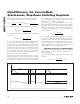
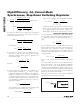
Figure 3. Asymptotic Loop Response of Current-Mode Regulator
GAIN
1ST ASYMPTOTE
R2 × (R1 + R2)
-1
× 10
AVEA(dB)/20
× g
MC
× R
LOAD
× {1 + R
LOAD
× [K
S
× (1 - D) - 0.5] × (L × f
SW
)
-1
}
-1
2ND ASYMPTOTE
R2 × (R1 + R2)
-1
× g
MV
× (2GC
C
)
-1
× g
MC
× R
LOAD
× {1 + R
LOAD
× [K
S
× (1 - D) - 0.5] × (L × f
SW
)
-1
}
-1
3RD ASYMPTOTE
R2 × (R1 + R2)
-1
× g
MV
× (2GC
C
)
-1
× g
MC
× R
LOAD
× {1 + R
LOAD
× [K
S
× (1 - D) - 0.5] × (L × f
SW
)
-1
}
-1
×
(2GC
OUT
× {R
LOAD
-1
+ [K
S
× (1 - D) - 0.5] × (L × f
SW
)
-1
}
-1
)
-1
4TH ASYMPTOTE
R2 × (R1 + R2)
-1
× g
MV
× R
C
× g
MC
× R
LOAD
× {1 + R
LOAD
× [K
S
× (1 - D) - 0.5] × (L × f
SW
)
-1
}
-1
×
(2GC
OUT
× {R
LOAD
-1
+ [K
S
× (1 - D) - 0.5] × (L × f
SW
)
-1
}
-1
)
-1
5TH ASYMPTOTE
R2 × (R1 + R2)
-1
× g
MV
× R
C
× g
MC
× R
LOAD
× {1 + R
LOAD
× [K
S
× (1 - D) - 0.5] × (L × f
SW
)
-1
}
-1
×
(2GC
OUT
× {R
LOAD
-1
+ [K
S
× (1 - D) - 0.5] × (L × f
SW
)
-1
}
-1
)
-1
× (0.5 × f
SW
)
2
× (2Gf)
-2
6TH ASYMPTOTE
R2 × (R1 + R2)
-1
× g
MV
× R
C
× g
MC
× R
LOAD
× {1 + R
LOAD
× [K
S
× (1 - D) - 0.5] × (L × f
SW
)
-1
}
-1
×
ESR × {R
LOAD
-1
+ [K
S
× (1 - D) - 0.5] × (L × f
SW
)
-1
}
-1
× (0.5 × f
SW
)
2
× (2Gf)
-2
UNITY
1ST POLE
[2GC
C
× (10
AVEA(dB)/20
- g
MV
-1
)]
-1
2ND POLE
f
PMOD
*
3RD POLE (DBL)
0.5 × f
SW
2ND ZERO
(2GC
OUT
ESR)
-1
FREQUENCY
f
CO
1ST ZERO
(2GC
C
R
C
)
-1
NOTE:
R
OUT
= 10
AVEA(dB)/20
× g
MV
-1
f
PMOD
= [2GC
OUT
× (ESR + {R
LOAD
-1
+ [K
S
× (1 - D) - 0.5] × (L × f
SW
)
-1
}
-1
)]
-1
WHICH FOR
ESR << {R
LOAD
-1
+ [K
S
× (1 - D) - 0.5] × (L × f
SW
)
-1
}
-1
BECOMES
f
PMOD
= [2GC
OUT
× {R
LOAD
-1
+ [K
S
× (1 - D) - 0.5] × (L × f
SW
)
-1
}
-1
]
-1
f
PMOD
= (2GC
OUT
× R
LOAD
)
-1
+ [K
S
× (1 - D) - 0.5] × (2GC
OUT
× L × f
SW
)
-1