User`s guide

The Simulink Environment
2-9
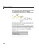
to produce a scalar output. Thus, the input to the Scope block is the
point-by-point sum of the two sinusoids.
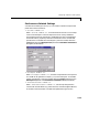
2 Double-click on the Scope block if the Scope window is not already open on
your screen. The scope window appears.
3 Select Start from the Simulation menu in the block diagram window. The
signal containing the summed 10 Hz and 20 Hz component sinusoids is
plotted on the scope.
4 Adjust the Scope block’s display.
a While the simulation is running, right-click on the y-axis of the scope and
select
Autoscale. The vertical range of the scope is adjusted to better fit
the signal.
b Click the Properties button on the scope, , and enter 0.1 for Time
range
. This resizes the scope’s time axis to display only one cycle of the
signal.
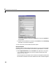
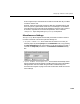
5 Vary the Sine Wave block parameters.
a While the simulation is running, double-click on the Sine Wave block to
open it.
b Change the frequencies of the two sinusoids. Try entering [1 5] or
[100 400] in the Frequency field. Press Apply after entering each new
value, and observe the changes on the scope.
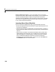
Note that the sample rate of both sinusoids is 1000 Hz, so aliasing will
occur for sinusoid frequencies above 500 Hz. You can increase the sample
rate by entering a smaller value in the Sine Wave block’s
Sample time
parameter. This parameter is not tunable (see below), so you will need to
stop the simulation before making any adjustment.
6 Select Stop from the Simulation menu to stop the simulation.
Many parameters cannot be changed while a simulation is running. This is
usually the case for parameters that directly or indirectly alter a signal’s
dimensions or sample rate. There are some parameters, however, like the Sine
Wave
Frequency parameter, that you can tune without terminating the
simulation. In the online “DSP Block Reference” these parameters are marked
“Tunable,” indicating that they are tunable while the simulation runs.