User`s guide

3 Fitting Data

3-18

conversion for a Type J thermocouple in the 0

to 760

temperature range is

described by a seventh-degree polynomial.

Note If you do not require a global parametric fit and want to maximize the

flexibility of the fit, piecewise polynomials might provide the best approach.

Refer to “Nonparametric Fitting” on page 3-68 for more information.

The main advantages of polynomial fits include reasonable flexibility for data

that is not too complicated, and they are linear, which means the fitting process

is simple. The main disadvantage is that high-degree fits can become unstable.

Additionally, polynomials of any degree can provide a good fit within the data

range, but can diverge wildly outside that range. Therefore, you should

exercise caution when extrapolating with polynomials. Refer to “Determining

the Best Fit” on page 1-8 for examples of good and poor polynomial fits to

census data.

Note that when you fit with high-degree polynomials, the fitting procedure

uses the predictor values as the basis for a matrix with very large values, which

can result in scaling problems. To deal with this, you should normalize the data

by centering it at zero mean and scaling it to unit standard deviation. You

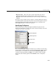
normalize data by selecting the

Center and scale X data check box on the

Fitting GUI.

Power Series

The toolbox provides a one-term and a two-term power series model.

Power series models are used to describe a variety of data. For example, the

rate at which reactants are consumed in a chemical reaction is generally

proportional to the concentration of the reactant raised to some power.

yax

yabx