User`s guide

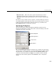
Parametric Fitting

3-17

For more information about the Fourier series, refer to “Fourier Analysis and

the Fast Fourier Transform” in the MATLAB documentation. For an example

that fits the ENSO data to a custom Fourier series model, refer to “General

Equation: Fourier Series Fit” on page 3-52.

Gaussian

The Gaussian model is used for fitting peaks, and is given by the equation

where a is the amplitude, b is the centroid (location), c is related to the peak

width, n is the number of peaks to fit, and .

Gaussian peaks are encountered in many areas of science and engineering. For

example, line emission spectra and chemical concentration assays can be

described by Gaussian peaks. For an example that fits two Gaussian peaks and

an exponential background, refer to “General Equation: Gaussian Fit with

Exponential Background” on page 3-57.

Polynomials

Polynomial models are given by

where n + 1 is the order of the polynomial, n is the degree of the polynomial,

and . The order gives the number of coefficients to be fit, and the

degree gives the highest power of the predictor variable.

In this guide, polynomials are described in terms of their degree. For example,

a third-degree (cubic) polynomial is given by

Polynomials are often used when a simple empirical model is required. The

model can be used for interpolation or extrapolation, or it can be used to

characterize data using a global fit. For example, the temperature-to-voltage

i 1=

∑

= e

–

-------------





–

1 n 8≤≤

n 1 i–+

i 1=

n 1+

∑

1 n 9≤≤

+++=