User`s guide

Parametric Fitting
3-11
The weights you supply should transform the response variances to a constant
value. If you know the variances of your data, then the weights are given by
If you don’t know the variances, you can approximate the weights using an
equation such as
This equation works well if your data set contains replicates. In this case, n is
the number of sets of replicates. However, the weights can vary greatly. A
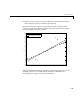
better approach might be to plot the variances and fit the data using a sensible
model. The form of the model is not very important — a polynomial or power
function works well in many cases.
Robust Least Squares
As described in “Basic Assumptions About the Error” on page 3-5, it is usually
assumed that the response errors follow a normal distribution, and that
extreme values are rare. Still, extreme values called outliers do occur.
The main disadvantage of least squares fitting is its sensitivity to outliers.
Outliers have a large influence on the fit because squaring the residuals
magnifies the effects of these extreme data points. To minimize the influence
of outliers, you can fit your data using robust least squares regression. The
toolbox provides these two robust regression schemes:
• Least absolute residuals (LAR) — The LAR scheme finds a curve that
minimizes the absolute difference of the residuals, rather than the squared
differences. Therefore, extreme values have a lesser influence on the fit.
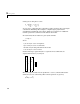
• Bisquare weights — This scheme minimizes a weighted sum of squares,
where the weight given to each data point depends on how far the point is
from the fitted line. Points near the line get full weight. Points farther from
w
i
1 σ
2
⁄=
w
i
1
n
---
y
i
y–()
2
i 1=
n
∑




1–
=