User`s guide

3 Fitting Data
3-8
Solving for b
2
using the b
1
value
As you can see, estimating the coefficients p
1
and p
2
requires only a few simple
calculations. Extending this example to a higher degree polynomial is
straightforward although a bit tedious. All that is required is an additional
normal equation for each linear term added to the model.
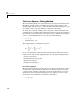
In matrix form, linear models are given by the formula
where
• y is an n-by-1 vector of responses.
• β is a m-by-1 vector of coefficients.
• X is the n-by-m design matrix for the model.
• ε is an n-by-1 vector of errors.
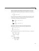
For the first-degree polynomial, the n equations in two unknowns are
expressed in terms of y, X, and β as
The least squares solution to the problem is a vector b, which estimates the
unknown vector of coefficients β. The normal equations are given by
b
2
1
n
---
y
i
b
1
x
i
∑
–
∑


=
yXβε+=
y
1
y
2
y
3
.
.
.
y
n
x
1
1
x
2
1
x
3
1
.
.
.
x
n
1
p
1
p
2
×=
X
T
X()bX
T
y=