User`s guide

3 Fitting Data
3-70
Note Goodness of fit statistics, prediction bounds, and weights are not
defined for interpolants. Additionally, the fit residuals are always zero (within
computer precision) because interpolants pass through the data points.
Interpolants are defined as piecewise polynomials because the fitted curve is
constructed from many “pieces.” For cubic spline and PCHIP interpolation,
each piece is described by four coefficients, which are calculated using a cubic
(third-degree) polynomial. Refer to the
spline function for more information
about cubic spline interpolation. Refer to the
pchip function for more
information about shape-preserving interpolation, and for a comparison of the
two methods.
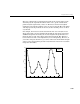
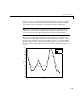
Parametric polynomial fits result in a global fit where one set of fitted
coefficients describes the entire data set. As a result, the fit can be erratic.
Because piecewise polynomials always produce a smooth fit, they are more
flexible than parametric polynomials and can be effectively used for a wider
range of data sets.
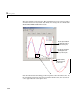
Smoothing Spline
If your data is noisy, you might want to fit it using a smoothing spline.
Alternatively, you can use one of the smoothing methods described in
“Smoothing Data” on page 2-9.
The smoothing spline s is constructed for the specified smoothing parameter p
and the specified weights w
i
. The smoothing spline minimizes
If the weights are not specified, they are assumed to be 1 for all data points.
p is defined between 0 and 1. p = 0 produces a least squares straight line fit to
the data, while p = 1 produces a cubic spline interpolant. If you do not specify
the smoothing parameter, it is automatically selected in the “interesting
range.” The interesting range of p is often near 1/(1+h
3
/6) where h is the
average spacing of the data points, and it is typically much smaller than the
allowed range of the parameter. Because smoothing splines have an associated
pw
i
y
i
( sx
i
())
2
– 1 p–()
x
2
2
d
d s



2
xd
∫
+
i
∑