User`s guide

Parametric Fitting
3-37
Example: Evaluating the Goodness of Fit
This example fits several polynomial models to generated data and evaluates
the goodness of fit. The data is cubic and includes a range of missing values.
rand('state',0)
x = [1:0.1:3 9:0.1:10]';
c = [2.5 -0.5 1.3 -0.1];
y = c(1) + c(2)*x + c(3)*x.^2 + c(4)*x.^3 + (rand(size(x))-0.5);
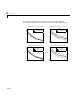
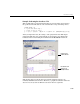
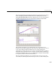
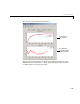
After you import the data, fit it using a cubic polynomial and a fifth degree
polynomial. The data, fits, and residuals are shown below. You display the
residuals in the Curve Fitting Tool with the
View->Residuals menu item.
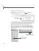
Both models appear to fit the data well, and the residuals appear to be
randomly distributed around zero. Therefore, a graphical evaluation of the fits
does not reveal any obvious differences between the two equations.
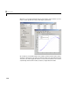
Both fits appear to
model the data well.
The residuals for both
fits appear to be
randomly distributed.