
User`s guide

Parametric Fitting
3-35
To understand the quantities associated with each type of prediction interval,
recall that the data, fit, and residuals (random errors) are related through the
formula
data = fit + residuals
Suppose you plan to take a new observation at the predictor value x
n+1
. Call
the new observation y
n+1
(x
n+1
) and the associated error e
n+1
. Then y
n+1
(x
n+1
)
satisfies the equation
where f
(x
n+1
) is the true but unknown function you want to estimate at x
n+1
.
The likely values for the new observation or for the estimated function are
provided by the nonsimultaneous prediction bounds.
If instead you want the likely value of the new observation to be associated
with any predictor value, the previous equation becomes
The likely values for this new observation or for the estimated function are
provided by the simultaneous prediction bounds.
The types of prediction bounds are summarized below.
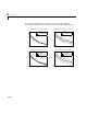
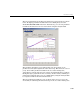
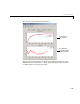
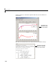
The nonsimultaneous and simultaneous prediction bounds for a new
observation and the fitted function are shown below. Each graph contains three
curves: the fit, the lower confidence bounds, and the upper confidence bounds.
The fit is a single-term exponential to generated data and the bounds reflect a
95% confidence level. Note that the intervals associated with a new observation
Table 3-3: Types of Prediction Bounds
Type of Bound Associated Equation
Observation Nonsimultaneous y
n+1
(x
n+1
)
Simultaneous y
n+1
(x), globally for any x
Function Nonsimultaneous f
(x
n+1
)
Simultaneous f(x), simultaneously for all x
y
n 1+
x
n 1+
()fx
n 1+
()e
n 1+
+=
y
n 1+
x() fx() e+=