User`s guide

3 Fitting Data
3-34
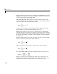
The nonsimultaneous prediction bounds for a new observation at the predictor
value x are given by
where s
2
is the mean squared error, t is the inverse of Student’s T cumulative
distribution function, and S is the covariance matrix of the coefficient
estimates, (X
T
X)
-1
s
2
. Note that x is defined as a row vector of the Jacobian
evaluated at a specified predictor value.
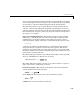
The simultaneous prediction bounds for a new observation and for all predictor
values are given by
where f is the inverse of the F cumulative distribution function. Refer to the
finv function, included with the Statistics Toolbox, for a description of f.
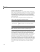
The nonsimultaneous prediction bounds for the function at a single predictor
value x are given by
The simultaneous prediction bounds for the function and for all predictor
values are given by
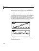
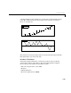
You can graphically display prediction bounds two ways: using the Curve
Fitting Tool or using the Analysis GUI. With the Curve Fitting Tool, you can
display nonsimultaneous prediction bounds for new observations with
View->Prediction Bounds. By default, the confidence level for the bounds is
95%. You can change this level to any value with
View->Confidence Level.
With the Analysis GUI, you can display nonsimultaneous prediction bounds for
the function or for new observations.
You can display numerical prediction bounds of any type at the command line
with the
predint function.
P
no,
y
ˆ
ts
2
xSx'+±=
P
so,
y
ˆ
fs
2
xSx'+±=
P
nf,
y
ˆ
txSx'±=
P
sf,
y
ˆ
fxSx'±=