
User`s guide
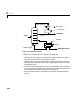
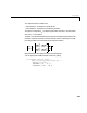
Table Of Contents
- Preface
- Quick Start
- LTI Models
- Introduction
- Creating LTI Models
- LTI Properties
- Model Conversion
- Time Delays
- Simulink Block for LTI Systems
- References
- Operations on LTI Models
- Arrays of LTI Models
- Model Analysis Tools
- The LTI Viewer
- Introduction
- Getting Started Using the LTI Viewer: An Example
- The LTI Viewer Menus
- The Right-Click Menus
- The LTI Viewer Tools Menu
- Simulink LTI Viewer
- Control Design Tools
- The Root Locus Design GUI
- Introduction
- A Servomechanism Example
- Controller Design Using the Root Locus Design GUI
- Additional Root Locus Design GUI Features
- References
- Design Case Studies
- Reliable Computations
- Reference
- Category Tables
- acker
- append
- augstate
- balreal
- bode
- c2d
- canon
- care
- chgunits
- connect
- covar
- ctrb
- ctrbf
- d2c
- d2d
- damp
- dare
- dcgain
- delay2z
- dlqr
- dlyap
- drmodel, drss
- dsort
- dss
- dssdata
- esort
- estim
- evalfr
- feedback
- filt
- frd
- frdata
- freqresp
- gensig
- get
- gram
- hasdelay
- impulse
- initial
- inv
- isct, isdt
- isempty
- isproper
- issiso
- kalman
- kalmd
- lft
- lqgreg
- lqr
- lqrd
- lqry
- lsim
- ltiview
- lyap
- margin
- minreal
- modred
- ndims
- ngrid
- nichols
- norm
- nyquist
- obsv
- obsvf
- ord2
- pade
- parallel
- place
- pole
- pzmap
- reg
- reshape
- rlocfind
- rlocus
- rltool
- rmodel, rss
- series
- set
- sgrid
- sigma
- size
- sminreal
- ss
- ss2ss
- ssbal
- ssdata
- stack
- step
- tf
- tfdata
- totaldelay
- zero
- zgrid
- zpk
- zpkdata
- Index

Time Delays
2-53
produces the discrete-time transfer function
Transfer function:
1
z^(–3) * -----------------
z^2 + 0.5 z + 0.2
Sampling time: 0.1
Notice the z^(–3) factor reflecting the three-sampling-period delay on the
input.
Mapping Discrete-Time Delays to Poles at the Origin
Since discrete-time delays are equivalent to additional poles at ,they can
be easily absorbed into the transfer function denominator or the state-space
equations. For example, the transfer function of the delayed integrator
is
You can specify this model either as the first-order transfer function
with a delay of two sampling periods on the input
Ts = 1; % sampling period
H1 = tf(1,[1 –1],Ts,'inputdelay',2)
or directly as a third-order transfer function:
H2 = tf(1,[1 –1 0 0],Ts) % 1/(z^3–z^2)
While these two models are mathematically equivalent, H1 is a more efficient
representation both in terms of storage and subsequent computations.
When necessary, you can map all discrete-time delays to poles at the origin
using the command
delay2z. For example,
H2 = delay2z(H1)
z 0
=
yk 1
+[]
yk
[]
uk 2
–[]+=
Hz()
z
2
–
z 1–
------------=
1 z 1
–()⁄