
User`s guide
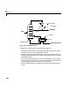
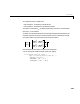
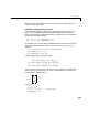
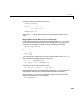
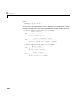
Table Of Contents
- Preface
- Quick Start
- LTI Models
- Introduction
- Creating LTI Models
- LTI Properties
- Model Conversion
- Time Delays
- Simulink Block for LTI Systems
- References
- Operations on LTI Models
- Arrays of LTI Models
- Model Analysis Tools
- The LTI Viewer
- Introduction
- Getting Started Using the LTI Viewer: An Example
- The LTI Viewer Menus
- The Right-Click Menus
- The LTI Viewer Tools Menu
- Simulink LTI Viewer
- Control Design Tools
- The Root Locus Design GUI
- Introduction
- A Servomechanism Example
- Controller Design Using the Root Locus Design GUI
- Additional Root Locus Design GUI Features
- References
- Design Case Studies
- Reliable Computations
- Reference
- Category Tables
- acker
- append
- augstate
- balreal
- bode
- c2d
- canon
- care
- chgunits
- connect
- covar
- ctrb
- ctrbf
- d2c
- d2d
- damp
- dare
- dcgain
- delay2z
- dlqr
- dlyap
- drmodel, drss
- dsort
- dss
- dssdata
- esort
- estim
- evalfr
- feedback
- filt
- frd
- frdata
- freqresp
- gensig
- get
- gram
- hasdelay
- impulse
- initial
- inv
- isct, isdt
- isempty
- isproper
- issiso
- kalman
- kalmd
- lft
- lqgreg
- lqr
- lqrd
- lqry
- lsim
- ltiview
- lyap
- margin
- minreal
- modred
- ndims
- ngrid
- nichols
- norm
- nyquist
- obsv
- obsvf
- ord2
- pade
- parallel
- place
- pole
- pzmap
- reg
- reshape
- rlocfind
- rlocus
- rltool
- rmodel, rss
- series
- set
- sgrid
- sigma
- size
- sminreal
- ss
- ss2ss
- ssbal
- ssdata
- stack
- step
- tf
- tfdata
- totaldelay
- zero
- zgrid
- zpk
- zpkdata
- Index

2 LTI Models
2-50
The resulti ng T F mod e l i s dis play ed as
Transfer function from input "R" to output...
12.8
Xd: exp(–1*s) * ----------
16.7 s + 1
6.6
Xb: exp(–7*s) * ----------
10.9 s + 1
Transfer function from input "S" to output...
–18.9
Xd: exp(–3*s) * --------
21 s + 1
–19.4
Xb: exp(–3*s) * ----------
14.4 s + 1
Specifying Delays on the Inputs or Outputs
While ideal for frequency-domain models with I/O delays, the ioDelayMatrix
property is inadequate to capture delayed inputs or outputs in state-space
models. For example, the two models
share the same transfer function
As a result, they cannot be distinguished using the
ioDelayMatrix property
(the I/O delay value is 0.1 seconds in both cases). Yet, these two models have
different state trajectories since and are related by
M
1
()
x
·
t() x– t() ut 0.1–()+=
yt() xt()=
M
2
()
z
·
t() z– t() ut()+=
yt() zt 0.1–()=
hs()
e
0.1s
–
s 1+
----------------=
xt
()
zt
()
zt
()
xt 0.1
–()=