
User`s guide
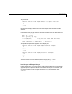
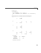
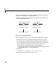
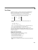

Table Of Contents
- Preface
- Quick Start
- LTI Models
- Introduction
- Creating LTI Models
- LTI Properties
- Model Conversion
- Time Delays
- Simulink Block for LTI Systems
- References
- Operations on LTI Models
- Arrays of LTI Models
- Model Analysis Tools
- The LTI Viewer
- Introduction
- Getting Started Using the LTI Viewer: An Example
- The LTI Viewer Menus
- The Right-Click Menus
- The LTI Viewer Tools Menu
- Simulink LTI Viewer
- Control Design Tools
- The Root Locus Design GUI
- Introduction
- A Servomechanism Example
- Controller Design Using the Root Locus Design GUI
- Additional Root Locus Design GUI Features
- References
- Design Case Studies
- Reliable Computations
- Reference
- Category Tables
- acker
- append
- augstate
- balreal
- bode
- c2d
- canon
- care
- chgunits
- connect
- covar
- ctrb
- ctrbf
- d2c
- d2d
- damp
- dare
- dcgain
- delay2z
- dlqr
- dlyap
- drmodel, drss
- dsort
- dss
- dssdata
- esort
- estim
- evalfr
- feedback
- filt
- frd
- frdata
- freqresp
- gensig
- get
- gram
- hasdelay
- impulse
- initial
- inv
- isct, isdt
- isempty
- isproper
- issiso
- kalman
- kalmd
- lft
- lqgreg
- lqr
- lqrd
- lqry
- lsim
- ltiview
- lyap
- margin
- minreal
- modred
- ndims
- ngrid
- nichols
- norm
- nyquist
- obsv
- obsvf
- ord2
- pade
- parallel
- place
- pole
- pzmap
- reg
- reshape
- rlocfind
- rlocus
- rltool
- rmodel, rss
- series
- set
- sgrid
- sigma
- size
- sminreal
- ss
- ss2ss
- ssbal
- ssdata
- stack
- step
- tf
- tfdata
- totaldelay
- zero
- zgrid
- zpk
- zpkdata
- Index
2 LTI Models
2-46
• Interconnections of continuous-time delay systems as long a s the resulting
transfer function from input to output is of t he form
where is a rational function of
• Padé approximation of time delays (
pade)
Specifying Input/Output Delays
Using the ioDelayMatrix property, you can specify frequency-domain models
with independent delays in each entry of the transfer function. In continuous
time, such models have a transfer function of the form
where the ’s are rational functions of , and is the time delay between
input andoutput . See “Specifying Delaysin Discrete-TimeModels”on page
2-52 for details on the discrete-time counterpart. We collectively refer to the
scalars as the I/O delays.
The syntax to create above is
H = tf(num,den,'iodelaymatrix',Tau)
or
H = zpk(z,p,k,'iodelaymatrix',Tau)
where
•
num,den (respectively,z,p,k)specify the rationalpart ofthe transfer
function
•
Tau is the matrix of time delays for each I/O pair. That is, Tau(i,j) specifies
the I/O delay in seconds. Note that
Tau and should have the same
row and column dimensions.
You can also use the
ioDelayMatrix property in conjunction with state-space
models, as in
sys = ss(A,B,C,D,'iodelaymatrix',Tau)
j
i
s
τ
ij
–()
h
ij
s
()
exp
h
ij
s
()
s
Hs()
e
sτ
11
–
h
11
s() ... e
sτ
1m
–
h
1m
s()
::
e
sτ
p1
–
h
p1
s() ... e
sτ
pm
–
h
pm
s()
sτ
ij
–()h
ij
s()exp[]==
h
ij
s
τ
ij
j
i
τ
ij
Hs
()
h
ij
s
()[]
Hs
()
τ
ij
Hs
()