
User`s guide
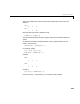
Table Of Contents
- Preface
- Quick Start
- LTI Models
- Introduction
- Creating LTI Models
- LTI Properties
- Model Conversion
- Time Delays
- Simulink Block for LTI Systems
- References
- Operations on LTI Models
- Arrays of LTI Models
- Model Analysis Tools
- The LTI Viewer
- Introduction
- Getting Started Using the LTI Viewer: An Example
- The LTI Viewer Menus
- The Right-Click Menus
- The LTI Viewer Tools Menu
- Simulink LTI Viewer
- Control Design Tools
- The Root Locus Design GUI
- Introduction
- A Servomechanism Example
- Controller Design Using the Root Locus Design GUI
- Additional Root Locus Design GUI Features
- References
- Design Case Studies
- Reliable Computations
- Reference
- Category Tables
- acker
- append
- augstate
- balreal
- bode
- c2d
- canon
- care
- chgunits
- connect
- covar
- ctrb
- ctrbf
- d2c
- d2d
- damp
- dare
- dcgain
- delay2z
- dlqr
- dlyap
- drmodel, drss
- dsort
- dss
- dssdata
- esort
- estim
- evalfr
- feedback
- filt
- frd
- frdata
- freqresp
- gensig
- get
- gram
- hasdelay
- impulse
- initial
- inv
- isct, isdt
- isempty
- isproper
- issiso
- kalman
- kalmd
- lft
- lqgreg
- lqr
- lqrd
- lqry
- lsim
- ltiview
- lyap
- margin
- minreal
- modred
- ndims
- ngrid
- nichols
- norm
- nyquist
- obsv
- obsvf
- ord2
- pade
- parallel
- place
- pole
- pzmap
- reg
- reshape
- rlocfind
- rlocus
- rltool
- rmodel, rss
- series
- set
- sgrid
- sigma
- size
- sminreal
- ss
- ss2ss
- ssbal
- ssdata
- stack
- step
- tf
- tfdata
- totaldelay
- zero
- zgrid
- zpk
- zpkdata
- Index

Creating LTI Models
2-21
produces
Transfer function:
z – 0.2
-------
z + 0.3
Sampling time: unspecified
Note: Do no t simply omit Ts in this case . This would make h a
continuous-time transfer function.
Ifyouforgettospecifythesampletimewhencreatingyourmodel,youcanstill
set it to the correct value by reassigning the LTI property
Ts. See “Sample
Time” on page 2-34 for more information on setting this property.
Discrete-Time TF and ZPK Models
Youcanspecifydiscrete-timeTFandZPKmodelsusingtf andzpk as indicated
above. Alternatively, it is often convenient to specify such models by:
1 Defining the variable z as a particular discrete-time TF or ZPK model with
theappropriatesampletime
2 Entering your TF or ZPK model directly as a rational e xpression in z.
This approach parallels the procedure for specifying continuous-time TF or
ZPK models using rational expressions. This procedure is described in “SISO
Transfer Function Models” on page 2-8 and “SISO Zero-Pole-Gain Models” on
page 2-12.
For example,
z = tf('z', 0.1);
H = (z+2)/(z^2 + 0.6*z + 0.9);
creates the same TF model as
H = tf([1 2], [1 0.6 0.9], 0.1);