
User`s guide
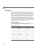
Table Of Contents
- Preface
- Quick Start
- LTI Models
- Introduction
- Creating LTI Models
- LTI Properties
- Model Conversion
- Time Delays
- Simulink Block for LTI Systems
- References
- Operations on LTI Models
- Arrays of LTI Models
- Model Analysis Tools
- The LTI Viewer
- Introduction
- Getting Started Using the LTI Viewer: An Example
- The LTI Viewer Menus
- The Right-Click Menus
- The LTI Viewer Tools Menu
- Simulink LTI Viewer
- Control Design Tools
- The Root Locus Design GUI
- Introduction
- A Servomechanism Example
- Controller Design Using the Root Locus Design GUI
- Additional Root Locus Design GUI Features
- References
- Design Case Studies
- Reliable Computations
- Reference
- Category Tables
- acker
- append
- augstate
- balreal
- bode
- c2d
- canon
- care
- chgunits
- connect
- covar
- ctrb
- ctrbf
- d2c
- d2d
- damp
- dare
- dcgain
- delay2z
- dlqr
- dlyap
- drmodel, drss
- dsort
- dss
- dssdata
- esort
- estim
- evalfr
- feedback
- filt
- frd
- frdata
- freqresp
- gensig
- get
- gram
- hasdelay
- impulse
- initial
- inv
- isct, isdt
- isempty
- isproper
- issiso
- kalman
- kalmd
- lft
- lqgreg
- lqr
- lqrd
- lqry
- lsim
- ltiview
- lyap
- margin
- minreal
- modred
- ndims
- ngrid
- nichols
- norm
- nyquist
- obsv
- obsvf
- ord2
- pade
- parallel
- place
- pole
- pzmap
- reg
- reshape
- rlocfind
- rlocus
- rltool
- rmodel, rss
- series
- set
- sgrid
- sigma
- size
- sminreal
- ss
- ss2ss
- ssbal
- ssdata
- stack
- step
- tf
- tfdata
- totaldelay
- zero
- zgrid
- zpk
- zpkdata
- Index

2 LTI Models
2-20
Discrete-Time Models
Creating discrete-time models is very much like creating continuous-time
models, exce p t that you must als o spe cif y a samp ling pe riod o r sample time for
discrete-timemodels.Thesampletimevalueshouldbescalarandexpressedin
seconds. Y ou c a n also us e the value –1 to leave t h e sample t ime unspecified.
To specif y discrete-time LTI models us ing
tf, zpk, ss,orfrd, simply append
the desired s amp le time value
Ts to the list of i nputs.
sys1 = tf(num,den,Ts)
sys2 = zpk(z,p,k,Ts)
sys3 = ss(a,b,c,d,Ts)
sys4 = frd(response,frequency,Ts)
For example,
h = tf([1 –1],[1 –0.5],0.1)
creates t he discrete-time transfer function with
sample time 0.1 seconds, and
sys = ss(A,B,C,D,0.5)
specifies the discrete-time state-space model
with sampling period 0.5 second. The vectors denote the
values of the state, input, and output vectors at the nth sample.
By convention, the sample time of continuous-time models is
Ts = 0.Setting
Ts = –1 leaves the sample time of a discrete-time model unspecified. For
example,
h = tf([1 –0.2],[1 0.3],–1)
hz
()
z 1
–()
z0.5
–()⁄=
xn 1
+[]
Ax n
[]
Bu n
[]+=
yn[] Cx n[] Du n[]+=
xn
[]
un
[]
yn
[],,