
User`s guide
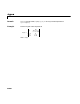


Table Of Contents
- Preface
- Quick Start
- LTI Models
- Introduction
- Creating LTI Models
- LTI Properties
- Model Conversion
- Time Delays
- Simulink Block for LTI Systems
- References
- Operations on LTI Models
- Arrays of LTI Models
- Model Analysis Tools
- The LTI Viewer
- Introduction
- Getting Started Using the LTI Viewer: An Example
- The LTI Viewer Menus
- The Right-Click Menus
- The LTI Viewer Tools Menu
- Simulink LTI Viewer
- Control Design Tools
- The Root Locus Design GUI
- Introduction
- A Servomechanism Example
- Controller Design Using the Root Locus Design GUI
- Additional Root Locus Design GUI Features
- References
- Design Case Studies
- Reliable Computations
- Reference
- Category Tables
- acker
- append
- augstate
- balreal
- bode
- c2d
- canon
- care
- chgunits
- connect
- covar
- ctrb
- ctrbf
- d2c
- d2d
- damp
- dare
- dcgain
- delay2z
- dlqr
- dlyap
- drmodel, drss
- dsort
- dss
- dssdata
- esort
- estim
- evalfr
- feedback
- filt
- frd
- frdata
- freqresp
- gensig
- get
- gram
- hasdelay
- impulse
- initial
- inv
- isct, isdt
- isempty
- isproper
- issiso
- kalman
- kalmd
- lft
- lqgreg
- lqr
- lqrd
- lqry
- lsim
- ltiview
- lyap
- margin
- minreal
- modred
- ndims
- ngrid
- nichols
- norm
- nyquist
- obsv
- obsvf
- ord2
- pade
- parallel
- place
- pole
- pzmap
- reg
- reshape
- rlocfind
- rlocus
- rltool
- rmodel, rss
- series
- set
- sgrid
- sigma
- size
- sminreal
- ss
- ss2ss
- ssbal
- ssdata
- stack
- step
- tf
- tfdata
- totaldelay
- zero
- zgrid
- zpk
- zpkdata
- Index

sigma
11-203
w = {wmin,wmax}. To use part icular frequency points, set w to the
corresponding vector of frequencies. Use
logspace to generate logarithmically
spaced frequency vectors. The frequencies must be specified in rad/sec.
sigma(sys,[],type) or sigma(sys,w,type) plots the following modified
singular value responses:
These options are available only for square systems, that is, with the same
number of inputs and outputs.
To superimpose the singular value plots of several LTI models on a single
figure, use
sigma(sys1,sys2,...,sysN)
sigma(sys1,sys2,...,sysN,[],type) % modified SV plot
sigma(sys1,sys2,...,sysN,w) % specify frequency range/grid
The models sys1,sys2,...,sysN need not have the same number of inputs
and outputs. Each model can be either continuous- or discrete-time. You can
also specify a distinctive color, linestyle, and/or marker for each system plot
with the syntax
sigma(sys1,'PlotStyle1',...,sysN,'PlotStyleN')
See bode for an example.
When invoked with output arguments,
[sv,w] = sigma(sys)
sv = sigma(sys,w)
return the singular values sv of t he frequency response at the frequencies w.
For a system with
Nu input and Ny outputs, the array sv has min(Nu,Ny) rows
and as many columns as frequency points (length of
w). The singular values at
the frequency
w(k) are given by sv(:,k).
type = 1
Singular values of t he frequency response , where is
the frequency response of
sys.
type = 2
Singular values of t he frequency response .
type = 3
Singular values of t he frequency response .
H
1
–
H
IH
+
IH
1
–
+