
User`s guide
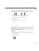
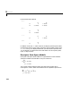
Table Of Contents
- Preface
- Quick Start
- LTI Models
- Introduction
- Creating LTI Models
- LTI Properties
- Model Conversion
- Time Delays
- Simulink Block for LTI Systems
- References
- Operations on LTI Models
- Arrays of LTI Models
- Model Analysis Tools
- The LTI Viewer
- Introduction
- Getting Started Using the LTI Viewer: An Example
- The LTI Viewer Menus
- The Right-Click Menus
- The LTI Viewer Tools Menu
- Simulink LTI Viewer
- Control Design Tools
- The Root Locus Design GUI
- Introduction
- A Servomechanism Example
- Controller Design Using the Root Locus Design GUI
- Additional Root Locus Design GUI Features
- References
- Design Case Studies
- Reliable Computations
- Reference
- Category Tables
- acker
- append
- augstate
- balreal
- bode
- c2d
- canon
- care
- chgunits
- connect
- covar
- ctrb
- ctrbf
- d2c
- d2d
- damp
- dare
- dcgain
- delay2z
- dlqr
- dlyap
- drmodel, drss
- dsort
- dss
- dssdata
- esort
- estim
- evalfr
- feedback
- filt
- frd
- frdata
- freqresp
- gensig
- get
- gram
- hasdelay
- impulse
- initial
- inv
- isct, isdt
- isempty
- isproper
- issiso
- kalman
- kalmd
- lft
- lqgreg
- lqr
- lqrd
- lqry
- lsim
- ltiview
- lyap
- margin
- minreal
- modred
- ndims
- ngrid
- nichols
- norm
- nyquist
- obsv
- obsvf
- ord2
- pade
- parallel
- place
- pole
- pzmap
- reg
- reshape
- rlocfind
- rlocus
- rltool
- rmodel, rss
- series
- set
- sgrid
- sigma
- size
- sminreal
- ss
- ss2ss
- ssbal
- ssdata
- stack
- step
- tf
- tfdata
- totaldelay
- zero
- zgrid
- zpk
- zpkdata
- Index

Creating LTI Models
2-15
Use the command ss to create state-space models
sys = ss(A,B,C,D)
For a model with Nx states, Ny out pu t s, and Nu inputs
•
A is an Nx-by-Nx real-valued m atrix.
•
B is an Nx-by-Nu real-v alued matrix.
•
C is an Ny-by-Nx real-v alued matri x.
•
D is an Ny-by-Nu real-v alued matri x.
This produces an SS object
sys that stores the state-space ma trice s
. For models with a zero D matrix, you can use
D = 0 (zero) as a
shorthand for a zero matrix of the appropriate dimensions .
As an illustration, consider the following simple model of an electric motor.
where is the angular displacement of the rotor and the driving current.
The relation between the input current and the angular velocity
is described by the state-space equations
where
This model is specified by typing
sys = ss([0 1;–5 –2],[0;3],[0 1],0)
ABCand D
,,,
d
2
θ
t
2
d
---------- 2
θd
td
------
5 θ++ 3I=
θ
I
uI
=
yd
θ
dt
⁄=
xd
td
------ Ax Bu+=
yCx=
x
θ
θd
td
------
= A
01
5– 2–
= B
0
3
= C
01
=