
User`s guide

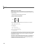
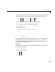
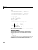
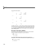
Table Of Contents
- Preface
- Quick Start
- LTI Models
- Introduction
- Creating LTI Models
- LTI Properties
- Model Conversion
- Time Delays
- Simulink Block for LTI Systems
- References
- Operations on LTI Models
- Arrays of LTI Models
- Model Analysis Tools
- The LTI Viewer
- Introduction
- Getting Started Using the LTI Viewer: An Example
- The LTI Viewer Menus
- The Right-Click Menus
- The LTI Viewer Tools Menu
- Simulink LTI Viewer
- Control Design Tools
- The Root Locus Design GUI
- Introduction
- A Servomechanism Example
- Controller Design Using the Root Locus Design GUI
- Additional Root Locus Design GUI Features
- References
- Design Case Studies
- Reliable Computations
- Reference
- Category Tables
- acker
- append
- augstate
- balreal
- bode
- c2d
- canon
- care
- chgunits
- connect
- covar
- ctrb
- ctrbf
- d2c
- d2d
- damp
- dare
- dcgain
- delay2z
- dlqr
- dlyap
- drmodel, drss
- dsort
- dss
- dssdata
- esort
- estim
- evalfr
- feedback
- filt
- frd
- frdata
- freqresp
- gensig
- get
- gram
- hasdelay
- impulse
- initial
- inv
- isct, isdt
- isempty
- isproper
- issiso
- kalman
- kalmd
- lft
- lqgreg
- lqr
- lqrd
- lqry
- lsim
- ltiview
- lyap
- margin
- minreal
- modred
- ndims
- ngrid
- nichols
- norm
- nyquist
- obsv
- obsvf
- ord2
- pade
- parallel
- place
- pole
- pzmap
- reg
- reshape
- rlocfind
- rlocus
- rltool
- rmodel, rss
- series
- set
- sgrid
- sigma
- size
- sminreal
- ss
- ss2ss
- ssbal
- ssdata
- stack
- step
- tf
- tfdata
- totaldelay
- zero
- zgrid
- zpk
- zpkdata
- Index

2 LTI Models
2-14
wher e
•
Z is the p -by-m cell array o f zero s (Z{i,j} = zeros of )
•
P is the p-by-m cell array o f p oles (P{i,j} = poles of )
•
K is the p -by-m matrix of g ains (K(i,j) = gain of )
For example, typing
Z = {[],–5;[1–i 1+i] []};
P = {0,[–1 –1];[1 2 3],[]};
K = [–1 3;2 0];
H = zpk(Z,P,K)
creates t he two-input/two-output zero-pole-gain model
Notice that you use
[] as a place-holder in Z (or P) when the corresponding
entry of has no zeros (or poles).
State-Space Models
State-space models rely on linear differential or difference equations to
describe the system dynamics. Continuous-time models are of the form
where x is the state vector and u and y are the input and output vectors. Such
models may arise from the equations of physics, from state-space
identification, or by state-space realization of the system transfer function.
H
ij
s
()
H
ij
s
()
H
ij
s
()
Hs()
1–
s
------
3 s 5+()
s1+()
2
--------------------
2 s
2
2 s– 2+()
s1–()s2–()s3–()
---------------------------------------------------
0
=
Hs
()
xd
td
------ Ax Bu+=
yCxDu+=