
User`s guide
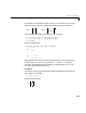
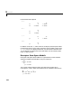
Table Of Contents
- Preface
- Quick Start
- LTI Models
- Introduction
- Creating LTI Models
- LTI Properties
- Model Conversion
- Time Delays
- Simulink Block for LTI Systems
- References
- Operations on LTI Models
- Arrays of LTI Models
- Model Analysis Tools
- The LTI Viewer
- Introduction
- Getting Started Using the LTI Viewer: An Example
- The LTI Viewer Menus
- The Right-Click Menus
- The LTI Viewer Tools Menu
- Simulink LTI Viewer
- Control Design Tools
- The Root Locus Design GUI
- Introduction
- A Servomechanism Example
- Controller Design Using the Root Locus Design GUI
- Additional Root Locus Design GUI Features
- References
- Design Case Studies
- Reliable Computations
- Reference
- Category Tables
- acker
- append
- augstate
- balreal
- bode
- c2d
- canon
- care
- chgunits
- connect
- covar
- ctrb
- ctrbf
- d2c
- d2d
- damp
- dare
- dcgain
- delay2z
- dlqr
- dlyap
- drmodel, drss
- dsort
- dss
- dssdata
- esort
- estim
- evalfr
- feedback
- filt
- frd
- frdata
- freqresp
- gensig
- get
- gram
- hasdelay
- impulse
- initial
- inv
- isct, isdt
- isempty
- isproper
- issiso
- kalman
- kalmd
- lft
- lqgreg
- lqr
- lqrd
- lqry
- lsim
- ltiview
- lyap
- margin
- minreal
- modred
- ndims
- ngrid
- nichols
- norm
- nyquist
- obsv
- obsvf
- ord2
- pade
- parallel
- place
- pole
- pzmap
- reg
- reshape
- rlocfind
- rlocus
- rltool
- rmodel, rss
- series
- set
- sgrid
- sigma
- size
- sminreal
- ss
- ss2ss
- ssbal
- ssdata
- stack
- step
- tf
- tfdata
- totaldelay
- zero
- zgrid
- zpk
- zpkdata
- Index

2 LTI Models
2-8
Creating LTI Models
The functions tf, zpk, ss,andfrd creat e transfer function models,
zero-pole-gain models, state-space models, and frequency response dat a
models,respectively.Thesefunctionst ake themodeldataas inputandproduce
TF, ZPK, SS, or FRD objects that store this data in a single MATLAB variable.
This section shows how to create continuous or discrete, SISO or MIMO LTI
models with
tf, zpk, ss,andfrd.
Note: You can only specify TF, ZPK, and SS models for systems whose
transfer matrices have re al -val ued coefficients.
Transfer Function Models
This sectio n explains ho w to spec if y continuous-time SISO and MIMO trans fer
function models. T he specification of discrete-time transfer function models i s
asimpleextensionofthecontinuous-timecase(see“Discrete-TimeModels”on
page 2-2 0) . In this s ect io n you can also read about how t o specify transfer
functions consisting of pure gains.
SISO Transfer Function Models
A continuous-time SISO transfer function
is cha racterized by its numerator and denominator , both
polynom ials of the Laplace variable s.
There are two ways to specify SISO transfer functions:
• Using the
tf command
• As rational expressio ns in t he Laplace variable s
To spe c ify a S I SO transfe r function model usin g the
tf
command, type
h = tf(num,den)
hs()
ns
()
ds()
-----------=
ns
()
ds
()
hs
()
ns
()
ds
()⁄=