
User`s guide
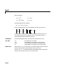
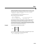
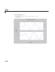
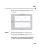
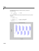
Table Of Contents
- Preface
- Quick Start
- LTI Models
- Introduction
- Creating LTI Models
- LTI Properties
- Model Conversion
- Time Delays
- Simulink Block for LTI Systems
- References
- Operations on LTI Models
- Arrays of LTI Models
- Model Analysis Tools
- The LTI Viewer
- Introduction
- Getting Started Using the LTI Viewer: An Example
- The LTI Viewer Menus
- The Right-Click Menus
- The LTI Viewer Tools Menu
- Simulink LTI Viewer
- Control Design Tools
- The Root Locus Design GUI
- Introduction
- A Servomechanism Example
- Controller Design Using the Root Locus Design GUI
- Additional Root Locus Design GUI Features
- References
- Design Case Studies
- Reliable Computations
- Reference
- Category Tables
- acker
- append
- augstate
- balreal
- bode
- c2d
- canon
- care
- chgunits
- connect
- covar
- ctrb
- ctrbf
- d2c
- d2d
- damp
- dare
- dcgain
- delay2z
- dlqr
- dlyap
- drmodel, drss
- dsort
- dss
- dssdata
- esort
- estim
- evalfr
- feedback
- filt
- frd
- frdata
- freqresp
- gensig
- get
- gram
- hasdelay
- impulse
- initial
- inv
- isct, isdt
- isempty
- isproper
- issiso
- kalman
- kalmd
- lft
- lqgreg
- lqr
- lqrd
- lqry
- lsim
- ltiview
- lyap
- margin
- minreal
- modred
- ndims
- ngrid
- nichols
- norm
- nyquist
- obsv
- obsvf
- ord2
- pade
- parallel
- place
- pole
- pzmap
- reg
- reshape
- rlocfind
- rlocus
- rltool
- rmodel, rss
- series
- set
- sgrid
- sigma
- size
- sminreal
- ss
- ss2ss
- ssbal
- ssdata
- stack
- step
- tf
- tfdata
- totaldelay
- zero
- zgrid
- zpk
- zpkdata
- Index

lsim
11-127
simulatestheresponsesofseveralLTI modelstothesameinputhistoryt,u and
plots these responses on a single figure. As with
bode or plot, you can specify
a particular color, linestyle, and/or marker for each system, for example,
lsim(sys1,'y:',sys2,'g--',u,t,x0)
The mult isystem behavior is similar to that of bode or step.
When i nvoked with left-hand arguments,
[y,t] = lsim(sys,u,t)
[y,t,x] = lsim(sys,u,t) % for state-space models only
[y,t,x] = lsim(sys,u,t,x0) % with initial state
return the output response y, the time vector t used for simulation, and the
state trajectories
x (for state-space models only). No plot is drawn on the
screen. The ma trix
y hasasmanyrowsastimesamples(length(t))andas
many columnsas systemoutputs.Thesame holds for
x with“outputs”replaced
bystates. Notethatthe output
t may differfrom the specified time vector when
the input data is undersampled (see “Algorithm”).
Example Simulate and plot the response of t he system
to a square wave with period of four seconds. First generate the square wave
with
gensig. Sample every 0.1 second during 10 seconds:
[u,t] = gensig('square',4,10,0.1);
Hs()
2s
2
5s 1++
s
2
2s3++
-------------------------------
s 1–
s
2
s 5++
------------------------
=