
User`s guide

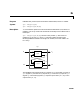
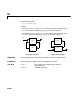
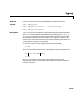
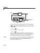
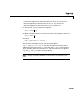
Table Of Contents
- Preface
- Quick Start
- LTI Models
- Introduction
- Creating LTI Models
- LTI Properties
- Model Conversion
- Time Delays
- Simulink Block for LTI Systems
- References
- Operations on LTI Models
- Arrays of LTI Models
- Model Analysis Tools
- The LTI Viewer
- Introduction
- Getting Started Using the LTI Viewer: An Example
- The LTI Viewer Menus
- The Right-Click Menus
- The LTI Viewer Tools Menu
- Simulink LTI Viewer
- Control Design Tools
- The Root Locus Design GUI
- Introduction
- A Servomechanism Example
- Controller Design Using the Root Locus Design GUI
- Additional Root Locus Design GUI Features
- References
- Design Case Studies
- Reliable Computations
- Reference
- Category Tables
- acker
- append
- augstate
- balreal
- bode
- c2d
- canon
- care
- chgunits
- connect
- covar
- ctrb
- ctrbf
- d2c
- d2d
- damp
- dare
- dcgain
- delay2z
- dlqr
- dlyap
- drmodel, drss
- dsort
- dss
- dssdata
- esort
- estim
- evalfr
- feedback
- filt
- frd
- frdata
- freqresp
- gensig
- get
- gram
- hasdelay
- impulse
- initial
- inv
- isct, isdt
- isempty
- isproper
- issiso
- kalman
- kalmd
- lft
- lqgreg
- lqr
- lqrd
- lqry
- lsim
- ltiview
- lyap
- margin
- minreal
- modred
- ndims
- ngrid
- nichols
- norm
- nyquist
- obsv
- obsvf
- ord2
- pade
- parallel
- place
- pole
- pzmap
- reg
- reshape
- rlocfind
- rlocus
- rltool
- rmodel, rss
- series
- set
- sgrid
- sigma
- size
- sminreal
- ss
- ss2ss
- ssbal
- ssdata
- stack
- step
- tf
- tfdata
- totaldelay
- zero
- zgrid
- zpk
- zpkdata
- Index

kalmd
11-112
11kalmd
Purpose Design discrete Kalman estimator for continuous plant
Syntax [kest,L,P,M,Z] = kalmd(sys,Qn,Rn,Ts)
Description kalmd designs a discrete-time Kalman estimator that has response
characteristics similar to a continuous-time estimator designed with
kalman.
This command is useful to derive a discrete estimator for digital
implementation after a satisfactory continuous estimator has been designed.
[kest,L,P,M,Z] = kalmd(sys,Qn,Rn,Ts) produces a discrete Kalman
estimator
kest with sample t ime Ts for the continuous-time plant
with process noise and measurement noise satis fying
The estimator
kest is derived a s follows. The continuous plant sys is first
discretized using zero-order hold with sample time
Ts (see c2d entry), and the
continuous noisecovariance matrices and arereplacedby theirdiscrete
equivalents
The integral is computed using the matrix exponential formulas in [2]. A
discrete-timeestimatoristhen designedforthe discretized plantandnoise.See
kalman for details on discrete-time Kalman estimation.
kalmd also returns the estimator gains L and M, and the discrete error
covariance matrices
P and Z (see kalman for details).
Limitations The discretized problem data should satisfy the requirements for kalman.
See Also kalman Design Kalman estimator
x
·
Ax Bu Gw++= (state equation)
y
v
Cx Du v++= (measurement equation)
w
v
Ew() Ev() 0, Eww
T
()Q
n
,= Evv
T
()R
n
=,Ewv
T
()0===
Q
n
R
n
Q
d
e
Aτ
GQG
T
e
A
T
τ
τd
0
T
s
∫
=
R
d
RT
s
⁄=