
User`s guide
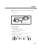
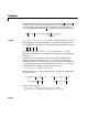
Table Of Contents
- Preface
- Quick Start
- LTI Models
- Introduction
- Creating LTI Models
- LTI Properties
- Model Conversion
- Time Delays
- Simulink Block for LTI Systems
- References
- Operations on LTI Models
- Arrays of LTI Models
- Model Analysis Tools
- The LTI Viewer
- Introduction
- Getting Started Using the LTI Viewer: An Example
- The LTI Viewer Menus
- The Right-Click Menus
- The LTI Viewer Tools Menu
- Simulink LTI Viewer
- Control Design Tools
- The Root Locus Design GUI
- Introduction
- A Servomechanism Example
- Controller Design Using the Root Locus Design GUI
- Additional Root Locus Design GUI Features
- References
- Design Case Studies
- Reliable Computations
- Reference
- Category Tables
- acker
- append
- augstate
- balreal
- bode
- c2d
- canon
- care
- chgunits
- connect
- covar
- ctrb
- ctrbf
- d2c
- d2d
- damp
- dare
- dcgain
- delay2z
- dlqr
- dlyap
- drmodel, drss
- dsort
- dss
- dssdata
- esort
- estim
- evalfr
- feedback
- filt
- frd
- frdata
- freqresp
- gensig
- get
- gram
- hasdelay
- impulse
- initial
- inv
- isct, isdt
- isempty
- isproper
- issiso
- kalman
- kalmd
- lft
- lqgreg
- lqr
- lqrd
- lqry
- lsim
- ltiview
- lyap
- margin
- minreal
- modred
- ndims
- ngrid
- nichols
- norm
- nyquist
- obsv
- obsvf
- ord2
- pade
- parallel
- place
- pole
- pzmap
- reg
- reshape
- rlocfind
- rlocus
- rltool
- rmodel, rss
- series
- set
- sgrid
- sigma
- size
- sminreal
- ss
- ss2ss
- ssbal
- ssdata
- stack
- step
- tf
- tfdata
- totaldelay
- zero
- zgrid
- zpk
- zpkdata
- Index
kalman
11-110
andgeneratesoptimal“current”outputandstateestimates and
using all available measurements including . The gain matrices and
are derived by solving a discrete Riccati equation. The innovation gain
is used to update the prediction using the new measurement .
Usage [kest,L,P] = kalman(sys,Qn,Rn,Nn) returns a state-space model kest of the
Kalman estimator given the plant model
sys and the noise covariance data Qn,
Rn, Nn (matrices above).sys must be a state-space model with matrices
The resulting estimator
kest has as inputs and (or their
discrete-time counterparts) as outputs. You can omit the last input argument
Nn when .
The function
kalman handles both continuous and discrete problems and
produces a continuous estimator when
sys is continuous, and a discrete
estimator otherwise. In continuous time,
kalman also returns the Kalman gain
L and the steady-state error covariance matrix P.NotethatPis the solution of
the associated Riccati equation. In discrete time, the syntax
[kest,L,P,M,Z] = kalman(sys,Qn,Rn,Nn)
returns the filte r gain and innovations gain , as well as the steady-state
error covariances
Finally, use the syntaxes
[kest,L,P] = kalman(sys,Qn,Rn,Nn,sensors,known)
[kest,L,P,M,Z] = kalman(sys,Qn,Rn,Nn,sensors,known)
y
ˆ
nn
[]
x
ˆ
nn
[]
y
v
n
[]
L
M
M
x
ˆ
nn 1–[]
y
v
n
[]
x
ˆ
nn[]x
ˆ
nn 1–[]My
v
n[] Cx
ˆ
nn 1–[]– Du n[]–
+=
innovation
QRN
,,
A
BG
C
DH
,,,
uy
v
;[] y
ˆ
;x
ˆ
[]
N0
=
L
M
PEenn1–[]enn 1–[]
T
(),
n∞→
lim= enn 1–[]xn[] xnn 1–[]–=
ZEenn[]enn[]
T
(),
n∞→
lim= enn[]xn[] xnn[]–=