
User`s guide
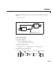
Table Of Contents
- Preface
- Quick Start
- LTI Models
- Introduction
- Creating LTI Models
- LTI Properties
- Model Conversion
- Time Delays
- Simulink Block for LTI Systems
- References
- Operations on LTI Models
- Arrays of LTI Models
- Model Analysis Tools
- The LTI Viewer
- Introduction
- Getting Started Using the LTI Viewer: An Example
- The LTI Viewer Menus
- The Right-Click Menus
- The LTI Viewer Tools Menu
- Simulink LTI Viewer
- Control Design Tools
- The Root Locus Design GUI
- Introduction
- A Servomechanism Example
- Controller Design Using the Root Locus Design GUI
- Additional Root Locus Design GUI Features
- References
- Design Case Studies
- Reliable Computations
- Reference
- Category Tables
- acker
- append
- augstate
- balreal
- bode
- c2d
- canon
- care
- chgunits
- connect
- covar
- ctrb
- ctrbf
- d2c
- d2d
- damp
- dare
- dcgain
- delay2z
- dlqr
- dlyap
- drmodel, drss
- dsort
- dss
- dssdata
- esort
- estim
- evalfr
- feedback
- filt
- frd
- frdata
- freqresp
- gensig
- get
- gram
- hasdelay
- impulse
- initial
- inv
- isct, isdt
- isempty
- isproper
- issiso
- kalman
- kalmd
- lft
- lqgreg
- lqr
- lqrd
- lqry
- lsim
- ltiview
- lyap
- margin
- minreal
- modred
- ndims
- ngrid
- nichols
- norm
- nyquist
- obsv
- obsvf
- ord2
- pade
- parallel
- place
- pole
- pzmap
- reg
- reshape
- rlocfind
- rlocus
- rltool
- rmodel, rss
- series
- set
- sgrid
- sigma
- size
- sminreal
- ss
- ss2ss
- ssbal
- ssdata
- stack
- step
- tf
- tfdata
- totaldelay
- zero
- zgrid
- zpk
- zpkdata
- Index

kalman
11-108
11kalman
Purpose Design continuous- or discrete-time Kalman estimator
Syntax [kest,L,P] = kalman(sys,Qn,Rn,Nn)
[kest,L,P,M,Z] = kalman(sys,Qn,Rn,Nn) % discrete time only
[kest,L,P] = kalman(sys,Qn,Rn,Nn,sensors,known)
Description kalman designs a Kalman state estimator given a state-space model of the
plant and the process and measurement noise covariance data. The Kalman
estimator is the optimal solution to the following continuous or discrete
estimation problems.
Continuous-Time Estimation
Given the continuous plant
with known inputs and process and measurement white noise
satisfying
construct a state estimate that minimizes the steady-state error
covariance
The optimal solution is the Kalman filter with equations
where thefilter gain is determined by solving an algebraic Riccati equation.
Thisestimator uses theknown inputs and the measurements togenerate
x
·
Ax Bu Gw++= (state equation)
y
v
Cx Du Hw v++ += (measurement equation)
u
wv
,
Ew() Ev() 0, Eww
T
()Q,= Evv
T
()R=,Ewv
T
()N===
x
ˆ
t()
PExx
ˆ
–{}xx
ˆ
–{}
T
()
t∞→
lim=
x
ˆ
·
Ax
ˆ
Bu L y
v
Cx
ˆ
– Du–()++=
y
ˆ
x
ˆ
C
I
x
ˆ
D
0
u+=
L
u
y
v