
User`s guide
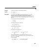


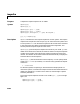
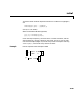
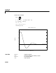
Table Of Contents
- Preface
- Quick Start
- LTI Models
- Introduction
- Creating LTI Models
- LTI Properties
- Model Conversion
- Time Delays
- Simulink Block for LTI Systems
- References
- Operations on LTI Models
- Arrays of LTI Models
- Model Analysis Tools
- The LTI Viewer
- Introduction
- Getting Started Using the LTI Viewer: An Example
- The LTI Viewer Menus
- The Right-Click Menus
- The LTI Viewer Tools Menu
- Simulink LTI Viewer
- Control Design Tools
- The Root Locus Design GUI
- Introduction
- A Servomechanism Example
- Controller Design Using the Root Locus Design GUI
- Additional Root Locus Design GUI Features
- References
- Design Case Studies
- Reliable Computations
- Reference
- Category Tables
- acker
- append
- augstate
- balreal
- bode
- c2d
- canon
- care
- chgunits
- connect
- covar
- ctrb
- ctrbf
- d2c
- d2d
- damp
- dare
- dcgain
- delay2z
- dlqr
- dlyap
- drmodel, drss
- dsort
- dss
- dssdata
- esort
- estim
- evalfr
- feedback
- filt
- frd
- frdata
- freqresp
- gensig
- get
- gram
- hasdelay
- impulse
- initial
- inv
- isct, isdt
- isempty
- isproper
- issiso
- kalman
- kalmd
- lft
- lqgreg
- lqr
- lqrd
- lqry
- lsim
- ltiview
- lyap
- margin
- minreal
- modred
- ndims
- ngrid
- nichols
- norm
- nyquist
- obsv
- obsvf
- ord2
- pade
- parallel
- place
- pole
- pzmap
- reg
- reshape
- rlocfind
- rlocus
- rltool
- rmodel, rss
- series
- set
- sgrid
- sigma
- size
- sminreal
- ss
- ss2ss
- ssbal
- ssdata
- stack
- step
- tf
- tfdata
- totaldelay
- zero
- zgrid
- zpk
- zpkdata
- Index

impulse
11-97
Because t his system has two inputs, y is a 3-D array with dimensions
size(y)
ans =
101 1 2
(the first dimension is the length of t). The impulse response of the first input
channel is then accessed by
y(:,:,1)
Algorithm Continuous-time models are first converted to state s pace. The impulse
response of a single-input state-space model
is equivalent to the following unforced response with init ial state .
To simulate this response, t he system is discretized using zero-order hold on
the inputs. The sampling period is chosen automatically based on the system
dynamics, except when a time vector
t = 0:dt:Tf is supplied (dt is then used
as sampling period).
Limitations Theimpulse responseofa continuoussystem with nonzero matrix isinfinite
at .
impulse ignores this discontinuity and returns the lower continuity
value at .
See Also ltiview LTIsystemviewer
step Step response
initial Free response to initial condition
lsim Simulate response to arbitrary inputs
x
·
Ax bu+=
yCx=
b
x
·
Ax ,= x 0() b=
yCx=
D
t0
=
Cb
t0
=