
User`s guide
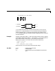
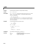
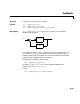
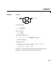
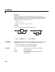
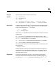
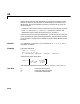
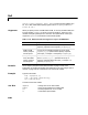
Table Of Contents
- Preface
- Quick Start
- LTI Models
- Introduction
- Creating LTI Models
- LTI Properties
- Model Conversion
- Time Delays
- Simulink Block for LTI Systems
- References
- Operations on LTI Models
- Arrays of LTI Models
- Model Analysis Tools
- The LTI Viewer
- Introduction
- Getting Started Using the LTI Viewer: An Example
- The LTI Viewer Menus
- The Right-Click Menus
- The LTI Viewer Tools Menu
- Simulink LTI Viewer
- Control Design Tools
- The Root Locus Design GUI
- Introduction
- A Servomechanism Example
- Controller Design Using the Root Locus Design GUI
- Additional Root Locus Design GUI Features
- References
- Design Case Studies
- Reliable Computations
- Reference
- Category Tables
- acker
- append
- augstate
- balreal
- bode
- c2d
- canon
- care
- chgunits
- connect
- covar
- ctrb
- ctrbf
- d2c
- d2d
- damp
- dare
- dcgain
- delay2z
- dlqr
- dlyap
- drmodel, drss
- dsort
- dss
- dssdata
- esort
- estim
- evalfr
- feedback
- filt
- frd
- frdata
- freqresp
- gensig
- get
- gram
- hasdelay
- impulse
- initial
- inv
- isct, isdt
- isempty
- isproper
- issiso
- kalman
- kalmd
- lft
- lqgreg
- lqr
- lqrd
- lqry
- lsim
- ltiview
- lyap
- margin
- minreal
- modred
- ndims
- ngrid
- nichols
- norm
- nyquist
- obsv
- obsvf
- ord2
- pade
- parallel
- place
- pole
- pzmap
- reg
- reshape
- rlocfind
- rlocus
- rltool
- rmodel, rss
- series
- set
- sgrid
- sigma
- size
- sminreal
- ss
- ss2ss
- ssbal
- ssdata
- stack
- step
- tf
- tfdata
- totaldelay
- zero
- zgrid
- zpk
- zpkdata
- Index
estim
11-71
estim handles both continuous- and discrete-time cases. You can use the
functions
place (pole placement) or kalman (Kalman filtering) to design an
adequate estimator gain . Note that the estimator poles (eigenvalues of
) should be faster than the plant dynamics (eigenvalues of ) to ensure
accurate estimation.
Example Consider a state-space model sys with seven outputs and four inputs. Suppose
you designed a Kalman gain matrix using outputs 4, 7, and 1 of the plant as
sensor measurements, and inputs 1,4, and 3 of the plant as known
(deterministic) inputs. You can then form the Kalma n estimator b y
sensors = [4,7,1];
known = [1,4,3];
est = estim(sys,L,sensors,known)
See the function kalman for direct Kalman e st imat or d e si gn.
See Also kalman Design Kalman estimator
place Pole placement
reg Form regulator given state-feedback and estimator
gains
x
ˆ
·
Ax
ˆ
B
2
uLyC
2
x
ˆ
D
22
u––()++=
y
ˆ
x
ˆ
C
2
I
x
ˆ
D
22
0
u+=
est
u (known)
y (sensors)
y
ˆ
x
ˆ
L
ALC
–
A
L