
User`s guide
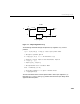
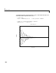

Table Of Contents
- Preface
- Quick Start
- LTI Models
- Introduction
- Creating LTI Models
- LTI Properties
- Model Conversion
- Time Delays
- Simulink Block for LTI Systems
- References
- Operations on LTI Models
- Arrays of LTI Models
- Model Analysis Tools
- The LTI Viewer
- Introduction
- Getting Started Using the LTI Viewer: An Example
- The LTI Viewer Menus
- The Right-Click Menus
- The LTI Viewer Tools Menu
- Simulink LTI Viewer
- Control Design Tools
- The Root Locus Design GUI
- Introduction
- A Servomechanism Example
- Controller Design Using the Root Locus Design GUI
- Additional Root Locus Design GUI Features
- References
- Design Case Studies
- Reliable Computations
- Reference
- Category Tables
- acker
- append
- augstate
- balreal
- bode
- c2d
- canon
- care
- chgunits
- connect
- covar
- ctrb
- ctrbf
- d2c
- d2d
- damp
- dare
- dcgain
- delay2z
- dlqr
- dlyap
- drmodel, drss
- dsort
- dss
- dssdata
- esort
- estim
- evalfr
- feedback
- filt
- frd
- frdata
- freqresp
- gensig
- get
- gram
- hasdelay
- impulse
- initial
- inv
- isct, isdt
- isempty
- isproper
- issiso
- kalman
- kalmd
- lft
- lqgreg
- lqr
- lqrd
- lqry
- lsim
- ltiview
- lyap
- margin
- minreal
- modred
- ndims
- ngrid
- nichols
- norm
- nyquist
- obsv
- obsvf
- ord2
- pade
- parallel
- place
- pole
- pzmap
- reg
- reshape
- rlocfind
- rlocus
- rltool
- rmodel, rss
- series
- set
- sgrid
- sigma
- size
- sminreal
- ss
- ss2ss
- ssbal
- ssdata
- stack
- step
- tf
- tfdata
- totaldelay
- zero
- zgrid
- zpk
- zpkdata
- Index

2 LTI Models
2-2
Introduction
The Control System Too lbox offers ex tensiv e to ols to manip ulate and anal yze
linear time-invariant (LTI) models. It supports b oth continuous- and
discrete - time systems. Systems ca n be si n gle- inp ut/s in g le-o u tpu t (S I SO) or
multiple-input/multiple-output(MIMO).In addition, you can store severalLTI
models in an arrayund er a single variable name. See Chapt er 4, “Arrays of LTI
Models” for inf ormati on o n L TI arrays.
This section introduceskey concepts about the MATLAB representation of LTI
models, including LTI objects, precedence rules for operations, and an analogy
between L TI systems and matrices. In addition, it summarizes the basic
commands you can use on LTI objects.
LTI Models
You can specify LTI models as:
• Transfer functions (TF), for example,
• Zero-pole-gain models (ZPK), for example,
• State- sp ace models (SS), for ex ample,
where A, B, C,andDare matrices of appropriate dimensions, x is the sta te
vector, and u and y are the input and output vectors.
• Frequency response data (FRD) models
FRD models consist of sampled measurements of a system’s frequency
response. For example, you can store experimentally collected frequency
response data in an FRD.
Ps()
s 2
+
s
2
s 10++
---------------------------=
Hz()
2z 0.5–()
zz 0.1+()
-------------------------
z
2
z 1++()
z0.2+()z0.1+()
---------------------------------------------
=
xd
td
------ Ax Bu+=
yCxDu+=