
User`s guide
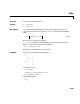
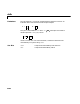
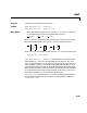
Table Of Contents
- Preface
- Quick Start
- LTI Models
- Introduction
- Creating LTI Models
- LTI Properties
- Model Conversion
- Time Delays
- Simulink Block for LTI Systems
- References
- Operations on LTI Models
- Arrays of LTI Models
- Model Analysis Tools
- The LTI Viewer
- Introduction
- Getting Started Using the LTI Viewer: An Example
- The LTI Viewer Menus
- The Right-Click Menus
- The LTI Viewer Tools Menu
- Simulink LTI Viewer
- Control Design Tools
- The Root Locus Design GUI
- Introduction
- A Servomechanism Example
- Controller Design Using the Root Locus Design GUI
- Additional Root Locus Design GUI Features
- References
- Design Case Studies
- Reliable Computations
- Reference
- Category Tables
- acker
- append
- augstate
- balreal
- bode
- c2d
- canon
- care
- chgunits
- connect
- covar
- ctrb
- ctrbf
- d2c
- d2d
- damp
- dare
- dcgain
- delay2z
- dlqr
- dlyap
- drmodel, drss
- dsort
- dss
- dssdata
- esort
- estim
- evalfr
- feedback
- filt
- frd
- frdata
- freqresp
- gensig
- get
- gram
- hasdelay
- impulse
- initial
- inv
- isct, isdt
- isempty
- isproper
- issiso
- kalman
- kalmd
- lft
- lqgreg
- lqr
- lqrd
- lqry
- lsim
- ltiview
- lyap
- margin
- minreal
- modred
- ndims
- ngrid
- nichols
- norm
- nyquist
- obsv
- obsvf
- ord2
- pade
- parallel
- place
- pole
- pzmap
- reg
- reshape
- rlocfind
- rlocus
- rltool
- rmodel, rss
- series
- set
- sgrid
- sigma
- size
- sminreal
- ss
- ss2ss
- ssbal
- ssdata
- stack
- step
- tf
- tfdata
- totaldelay
- zero
- zgrid
- zpk
- zpkdata
- Index

d2c
11-49
As with zero-order hold, the inverse discretization operation
c2d(Hc,0.1,'tustin')
gives back the original .
Algorithm The 'zoh' conversion is performed in state space and relies on the matrix
logarithm (see
logm in Using MATLAB).
Limitations The Tustin approximation is not defined for systems with poles at and
is ill-conditioned for systems with poles near .
The zero-order hold method cannot handle systems with poles at . In
addition, the
'zoh' conversion increases the model order for systems with
negative real poles, [2]. This is necessary because the matrix logarithm maps
real negative poles to complex poles. As a result,a discrete model with a single
pole at would be transformed to a continuous model with a single
complex pole at . Such a model is not meaningful
because of it s complex time response.
To ensure that all complex poles of the continuous model come in conjugate
pairs,
d2c replaces negative real poles with a pair of complex conjugate
poles near . The conversion then yields a continuous model with higher
order. For example, the discrete model with transfer function
and sample time 0.1 second is converted by typing
Ts = 0.1
H = zpk(–0.2,–0.5,1,Ts) * tf(1,[1 1 0.4],Ts)
Hc = d2c(H)
MATLAB responds with
Warning: System order was increased to handle real negative poles.
Zero/pole/gain:
–33.6556 (s–6.273) (s^2 + 28.29s + 1041)
--------------------------------------------
(s^2 + 9.163s + 637.3) (s^2 + 13.86s + 1035)
Hz
()
z 1
–=
z 1
–=
z 0
=
z 0.5
–=
0.5
–()
log 0.6931
–
j
π+≈
z
α–=
α–
Hz()
z 0.2
+
z 0.5+()z
2
z0.4++()
---------------------------------------------------------=