
User`s guide
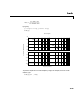
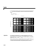
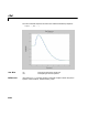
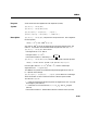
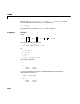
Table Of Contents
- Preface
- Quick Start
- LTI Models
- Introduction
- Creating LTI Models
- LTI Properties
- Model Conversion
- Time Delays
- Simulink Block for LTI Systems
- References
- Operations on LTI Models
- Arrays of LTI Models
- Model Analysis Tools
- The LTI Viewer
- Introduction
- Getting Started Using the LTI Viewer: An Example
- The LTI Viewer Menus
- The Right-Click Menus
- The LTI Viewer Tools Menu
- Simulink LTI Viewer
- Control Design Tools
- The Root Locus Design GUI
- Introduction
- A Servomechanism Example
- Controller Design Using the Root Locus Design GUI
- Additional Root Locus Design GUI Features
- References
- Design Case Studies
- Reliable Computations
- Reference
- Category Tables
- acker
- append
- augstate
- balreal
- bode
- c2d
- canon
- care
- chgunits
- connect
- covar
- ctrb
- ctrbf
- d2c
- d2d
- damp
- dare
- dcgain
- delay2z
- dlqr
- dlyap
- drmodel, drss
- dsort
- dss
- dssdata
- esort
- estim
- evalfr
- feedback
- filt
- frd
- frdata
- freqresp
- gensig
- get
- gram
- hasdelay
- impulse
- initial
- inv
- isct, isdt
- isempty
- isproper
- issiso
- kalman
- kalmd
- lft
- lqgreg
- lqr
- lqrd
- lqry
- lsim
- ltiview
- lyap
- margin
- minreal
- modred
- ndims
- ngrid
- nichols
- norm
- nyquist
- obsv
- obsvf
- ord2
- pade
- parallel
- place
- pole
- pzmap
- reg
- reshape
- rlocfind
- rlocus
- rltool
- rmodel, rss
- series
- set
- sgrid
- sigma
- size
- sminreal
- ss
- ss2ss
- ssbal
- ssdata
- stack
- step
- tf
- tfdata
- totaldelay
- zero
- zgrid
- zpk
- zpkdata
- Index
bode
11-22
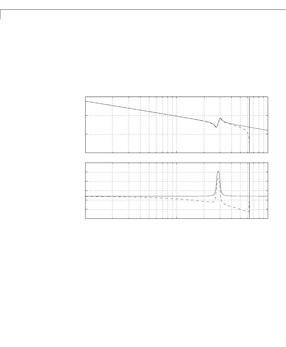
You can also discretize this system using zero-order hold and the sample time
second, and compare the continuous and discretized responses by
typing
gd = c2d(g,0.5)
bode(g,'r',gd,'b--')
Algorithm For continuous-time systems, bode computes t he frequency response by
evaluating the transfer function on the imaginary axis . Only
positive frequencies are considered. For state-space models, the frequency
response is
When numerical ly safe, is diagonalized for maximum speed. Otherwise,
is reduced to upper Hessenberg form and the linear equation
is solved at each frequency point, taking advantage of the Hessenberg
T
s
0.5
=
Frequency (rad/sec)
Phase (deg); Magnitude (dB)
Bode Diagrams
−100
−50
0
50
10
−1
10
0
10
1
−300
−250
−200
−150
−100
−50
0
Hs
()
sj
ω=
ω
DCjωA–()
1
–
B+ ,ω0≥
A
A
j
ω
A
–()
XB
=